EP 112
What Happens Inside an AI Chip: From KV Cache to Roofline
Value Capture Shifting to AI Infrastructure 0:00

Chester Roh Today, as we’re recording, is August 30th, 2026, a Sunday morning. Today, we have HyperAccel CTO Jinwon Lee with us. There has been so much news lately, right? But if we arrange the news by category, from data centers at the bottom to chips and models, and then applications on top, there are various layers, and lately, what I’ve been noticing is that progress on the model side is happening so quickly that, as they call it, value capture— the areas that actually make money— is moving down toward infrastructure, and moving up toward applications, and we’ve been seeing these two trends. Today, we’re going to hear a very important lesson from our guest. It’s about this lower layer. We put power into building chips, load trained models onto them, and provide customers with an enormous amount of inference, after all. What is happening inside that, and what we need to understand to read the benchmarks within it—we previously covered inference with Seungjoon, armed with this shallow knowledge, while doing Dwarkesh’s roofline analysis, and talked about inference once, and since then, we’ve been discussing inference very frequently. The reason we talk about it so often is probably because it is so important. Today is the ultimate masterclass edition of that. If you carefully follow CTO Jinwon Lee’s lecture, you’ll be able to understand the various new benchmarks coming out of SemiAnalysis, the things NVIDIA announces, and the things chip companies announce as well. That’s why. Let’s invite CTO Jinwon Lee and hear from him. Welcome, CTO Lee.
Jinwon Lee Hello. Nice to meet you. It’s been a while since I last appeared.
Chester Roh Today’s content is really, really deep and extensive. So no matter how long it takes, I hope you’ll teach us carefully. We’re counting on you.
Seungjoon Choi Wasn’t it May when we talked about Dwarkesh? Already?
Chester Roh About three months have passed, but even in that time, since it’s three months in the AI world, we should consider it three years.
Perpetual Compute Shortages and Exploding Token Demand 2:13
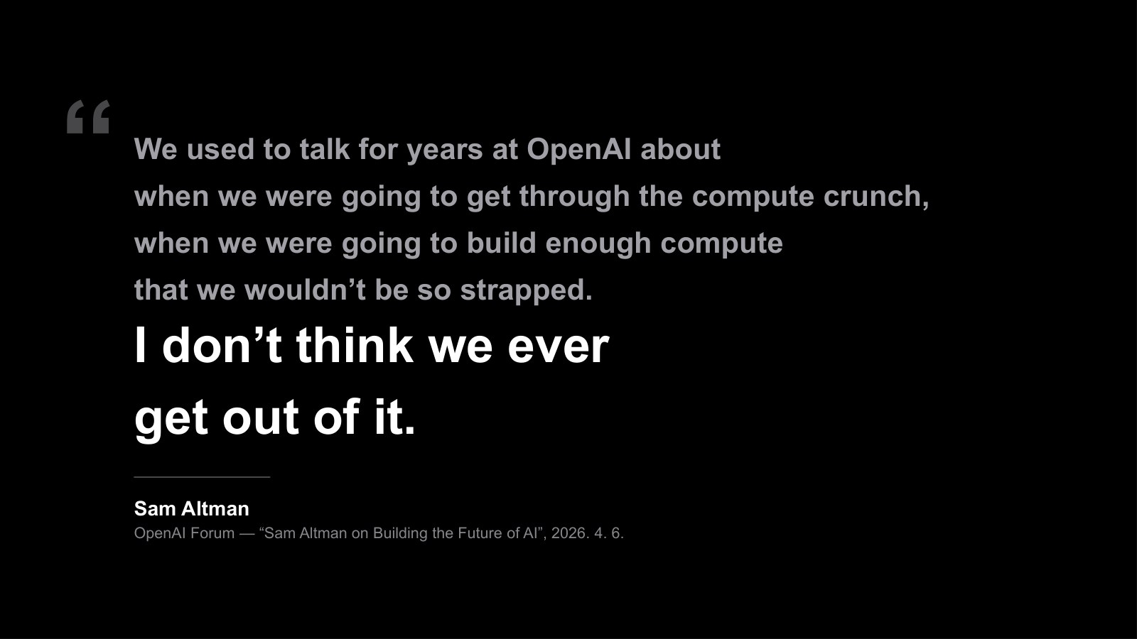
Jinwon Lee Shall we get started? What I’ll be discussing today is related to inference engineering. You all are probably using AI very extensively now, but on the GPUs mainly used or other AI semiconductors, what exactly is happening is difficult material, but I’ll explain it as simply as possible today. I’ll first talk about matters related to our company, and then we’ll begin in earnest. This is something Sam Altman said at the OpenAI Forum in April this year. If you look here, it says “compute crunch”: we live in a world where compute is severely lacking, and when will we be able to escape from that? This is something OpenAI people have discussed for years, but at this point, it seems that going forward, we may never escape it. In other words, we will always live in a world short of compute, is what he is saying. Whether for training or inference, we are in a situation where compute is insufficient.
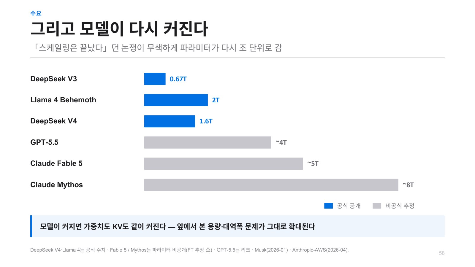
Another thing that shows this well was announced at Google I/O in May: after examining token usage on GCP, Google announced that monthly usage had increased fiftyfold in twelve months. And last September, I went to the AI Infrastructure Summit, where Google also gave a presentation, saying that it had doubled again in just two months and become one hundred times larger in fourteen months. And what has happened now? It has increased significantly again since then, to roughly 330 times the level in 2024, and they continue to say that there is enormous explosive demand. As everyone knows, models are also continuing to grow. What is shown here includes unofficial estimates, and I recently heard that Fable 5 has around 8T parameters, as well, and for a while, models appeared not to be growing much, as if they were not getting bigger beyond several trillion parameters, but Mythos is rumored to have 10T parameters, so model scale is growing again as well.
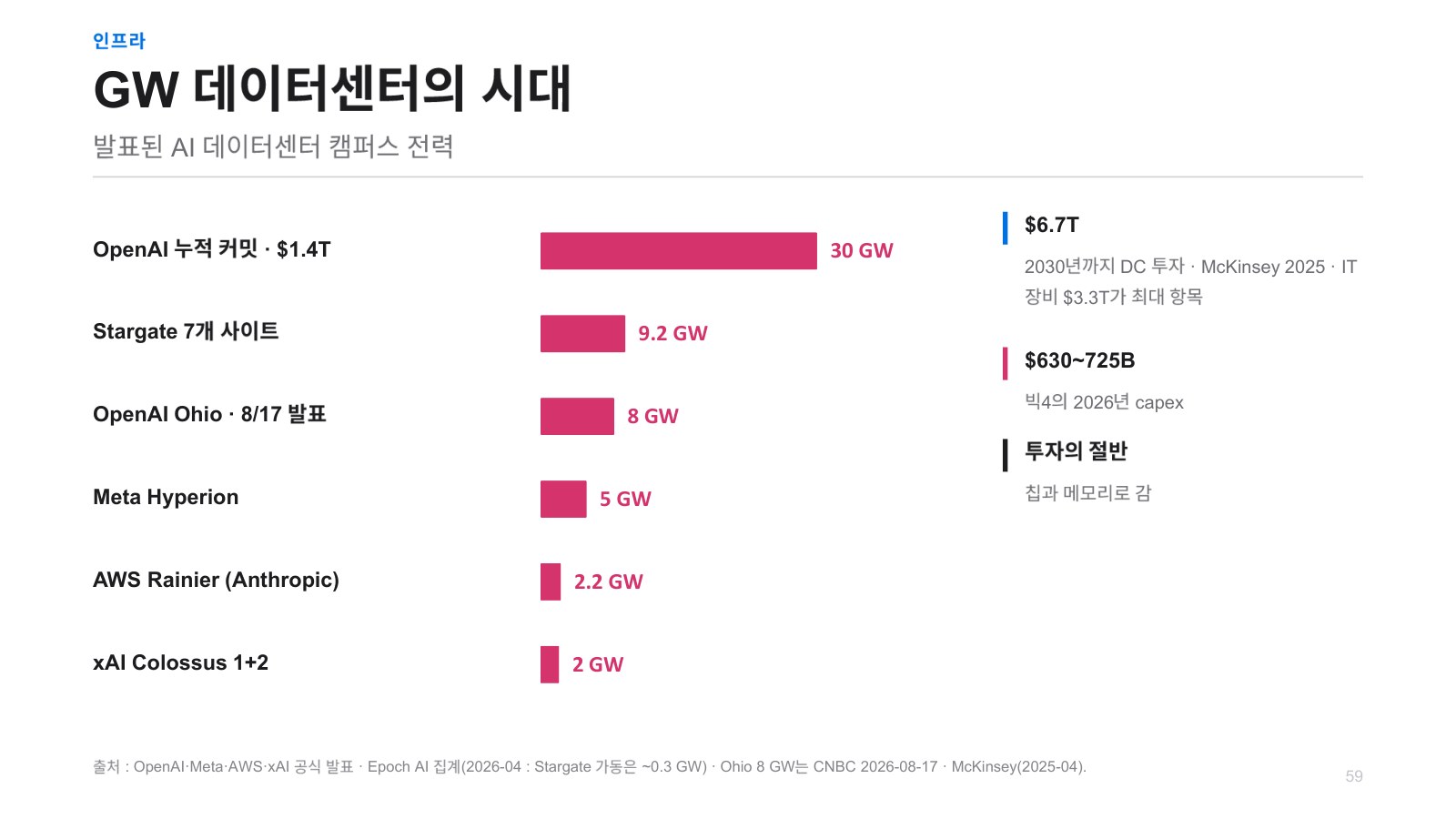
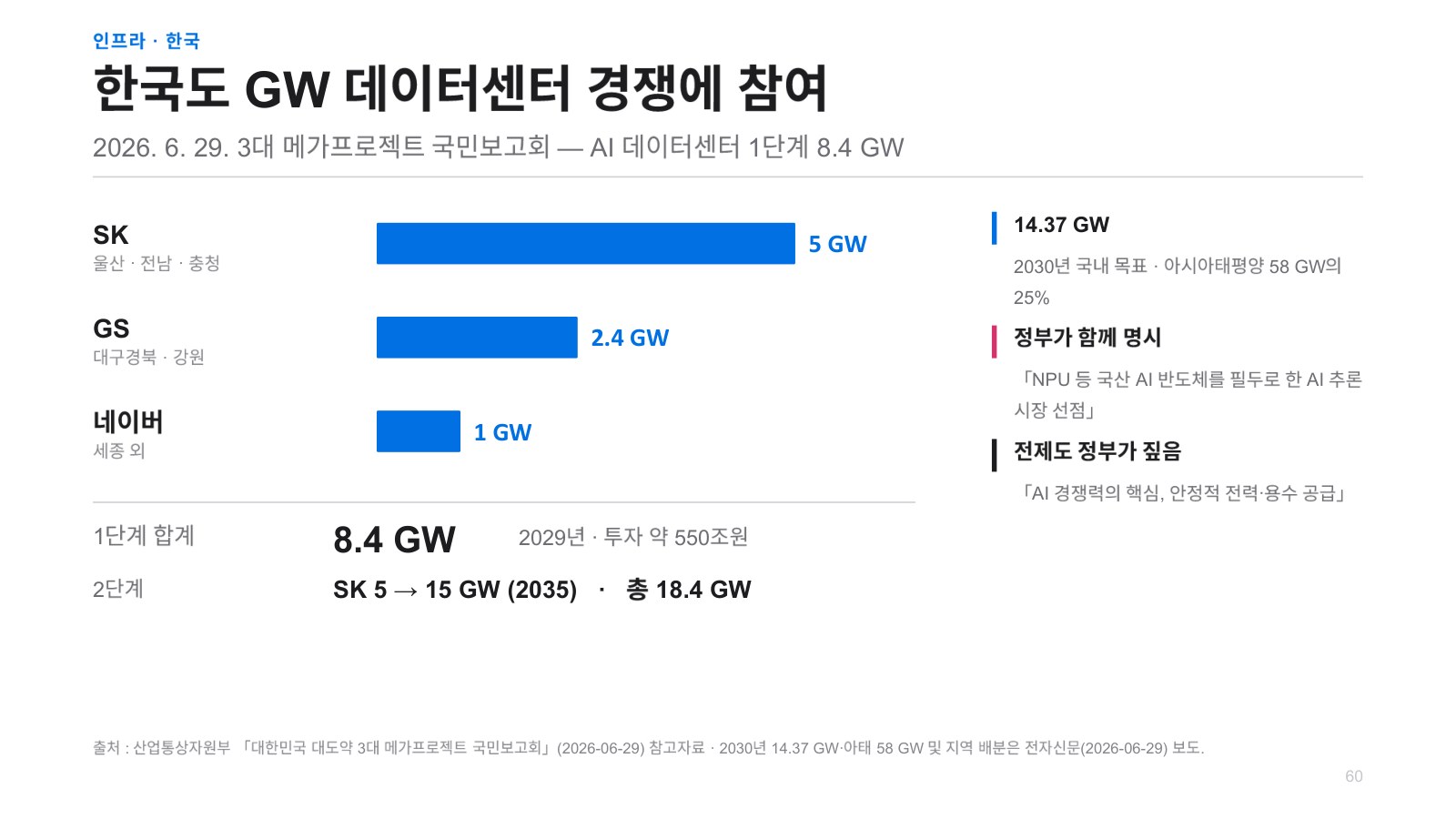
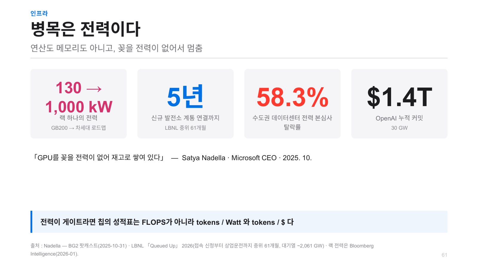
And to handle this, data centers are being built at an enormous scale worldwide. They’re called GW data centers, and if you look here, by 2030, about $6.7 trillion will be spent on data centers, which, in Korean won, comes to nearly 10 quadrillion won. And in Korea as well, there are currently four mega-projects, aiming to build 18.4 GW worth of data centers on Korean soil by 2035. As this happens, as everyone often says, electricity is the problem. Everyone is talking about how to supply power, and here, when data centers are built in the United States, until electricity is connected to them, it takes about five years on average. And when data center power applications are reviewed in Korea’s Seoul metropolitan area, more than half of them fail, according to reports that keep coming out. So power is a huge issue, and another thing that came up on the Dwarkesh podcast was that Anthropic has now been growing its revenue tenfold for three consecutive years, while these frontier labs are increasing compute, meaning computational capacity, by three times each year.
Revenue–Compute Gaps Driving Up Inference Unit Costs 5:17
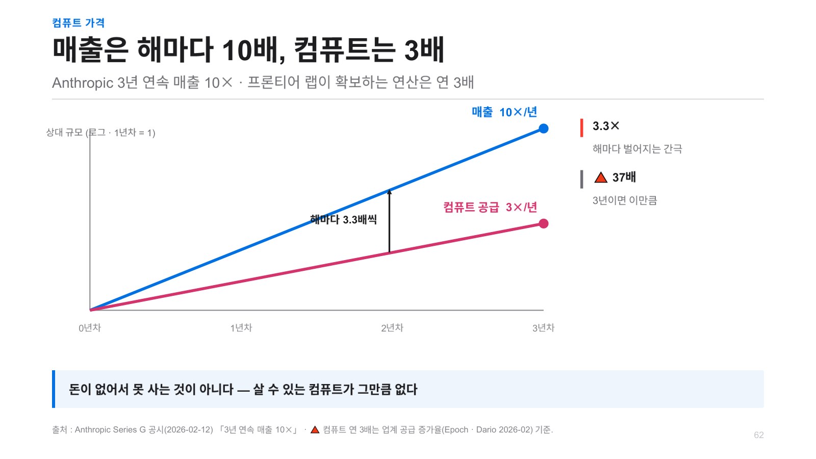

Jinwon Lee That means the gap widens by 3.3 times a year. So GPU compute increases threefold, while revenue grows tenfold. How should we interpret this gap? There are three ways to do so. First, during inference, they could raise margins to increase revenue. But Anthropic’s inference margin is already reportedly 70–80%, and if we assume the ceiling is 90%, there is hardly any room left to increase it. And second, if I have 100 GPUs, 100 units, and am currently using 70 of them for training and 30 for service, I could increase that ratio to 50–50 and raise the share of GPUs used for inference, which would generate revenue, so with the same compute, that would be a way to increase revenue. But it is currently known to be roughly 50–50, and many people say it would be difficult to increase this further. Because reducing the share used for training means putting less effort into model development, and these frontier labs right now are in a situation where survival is difficult. So it is difficult to raise this much as well. Then what remains is, ultimately, that the unit price of compute can only go up. So neocloud companies and companies like them are also making very strong profits, and for short-term rentals, you have to pay more than twice as much as for long-term rentals, so in this way, the actual unit price of compute is also rising significantly.
HyperAccel Bertha Chip Choosing LPDDR over HBM 7:17
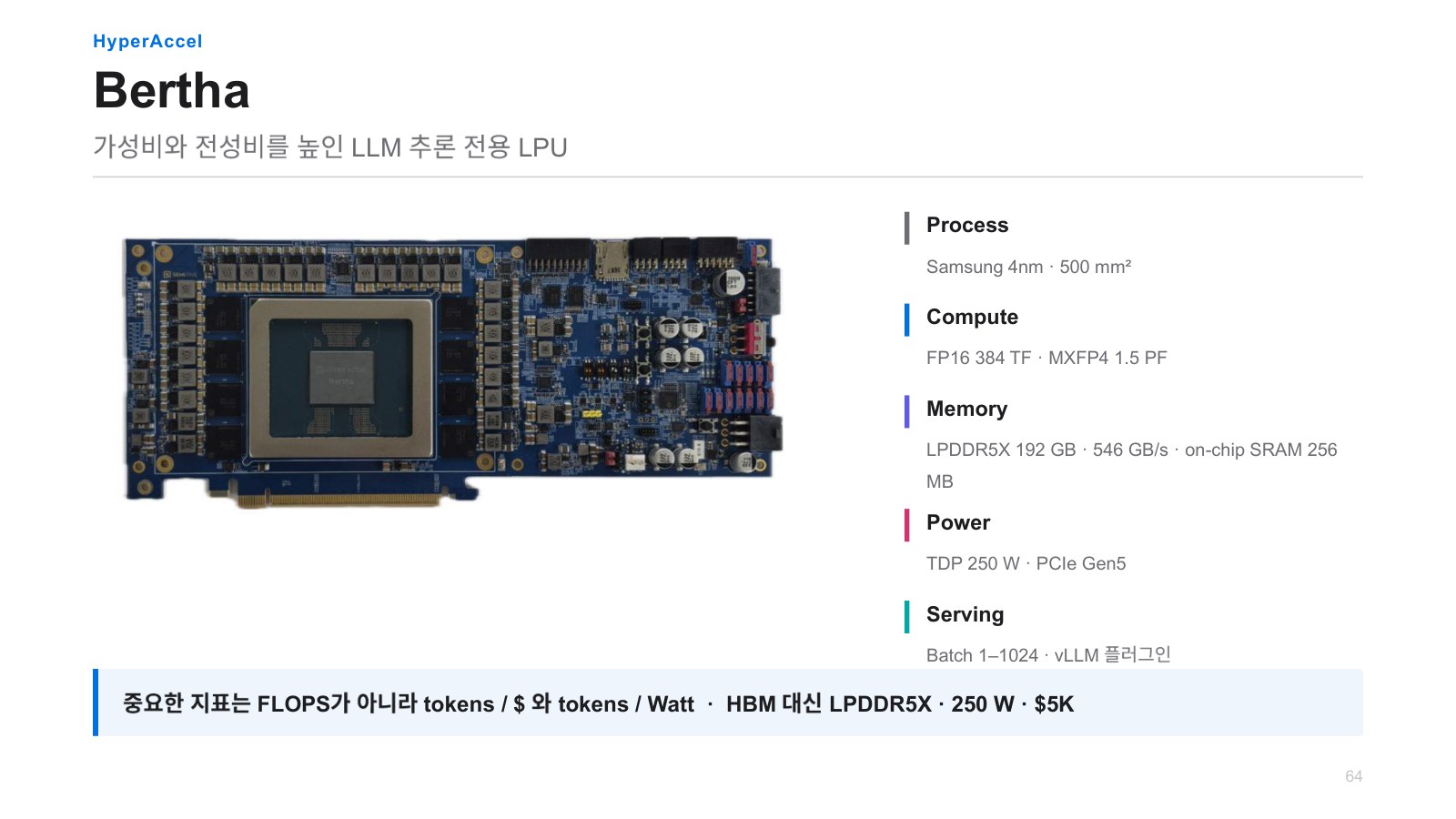
Jinwon Lee So the reason I laid out this background first is that the chip we are making is called Bertha. This is our first, the first one made by our company: a data center-class AI chip. The distinguishing feature of our product is that, instead of using the HBM everyone uses, it uses low-power DDR memory called LPDDR. What we can gain from this is lower power consumption compared with chips that use HBM. And above all, HBM is very expensive and difficult to obtain, whereas we use DDR, so we can supply it at a very low cost. So we planned and developed a product that can dramatically reduce the cost of the AI services you use. It is currently manufactured using Samsung’s 4nm process, and this chip came out at the end of March this year, so we are now working hard on bring-up.
Bring-up means loading software onto the chip and getting it to a level where it can provide services. We did demonstrate it at Hot Chips, which was held last week. After refining it a little more, and within a month or two, we plan to release it widely to the market for PoC purposes. So our chip is a very affordable, low-power chip; I hope you will remember it that way.
Bandwidth Secured with LPDDR and a $5,000 Target Price 8:42
Jonghyun Park You mentioned that you use LPDDR, and the reason HBM is used so much is that memory bandwidth is important, and it is difficult to increase memory bandwidth with LPDDR. So even with LPDDR, is there some method that increases memory bandwidth, or have other things been applied?
Jinwon Lee If you look at our PCIe card here, these are LPDDR memories. You can see that there are eight of them, with four attached on each side. First of all, we put in a great deal of DDR. There are only a few chips like this anywhere in the world. There are chips made by NVIDIA or previously by Meta. So by putting in a lot of DDR, we secured a certain amount of bandwidth.
Another, and most important, point is that our company’s architecture can utilize more than 90% of the bandwidth through its internal architecture. So our bandwidth right now is listed as 546GB/s, while GPUs like the H100 have around 3TB/s. So that is about one-sixth, but that is a theoretical figure, and when you actually load and run an AI workload, if you measure how much of this bandwidth is actually used as utilization, without any optimization, it comes out to around 50%, and with extensive optimization, it can rise to around 70%. But we have an architecture that achieves over 90%, so we can overcome that to some extent.
So how cheap is it? Our current target price is about $5,000, so Compared with GPU prices, you can see that it is extremely affordable. That comes to under 10 million Korean won. And because we use DDR for memory capacity as well, we have 192GB per chip, so with a small number of chips, we also have the advantage of being able to serve large models.
Chester Roh As we have continued to explain the background earlier, demand is constantly increasing, so making chips of this kind will continue to be meaningful for quite some time.
Jinwon Lee As demand grows, application requirements are also extremely diverse, and as I will explain again later, bandwidth is directly connected to speed. If bandwidth is low, speeds can be a little slower, but speed is not that important for some applications, and there are a great many of them, so because our costs are low, we think we will be a good fit for that market as well.
Chester Roh When we work with ChatGPT, we spend most of our time reading text and waiting, so those inefficiencies in this inference market will accumulate as they are.
Origin of the Name LPU and OpenAI Jalapeño 11:29
Seungjoon Choi What is an LPU? Can it be used on its own? Or is it a component that goes into something larger?
Jinwon Lee Coincidentally, Groq, which NVIDIA acquired, also uses the name LPU, and we also use the name LPU, but we actually used the name LPU much earlier. Groq was originally called TSP, Tensor Streaming Processor, and later changed its name to LPU. But because Groq’s LPU is better known, people often ask what an LPU is and whether it is another new kind of NPU, but it is just a name. Broadly speaking, they are all just types of NPU, and ours can operate independently. GPUs also come as PCIe card products, right? You can think of it as the same thing.
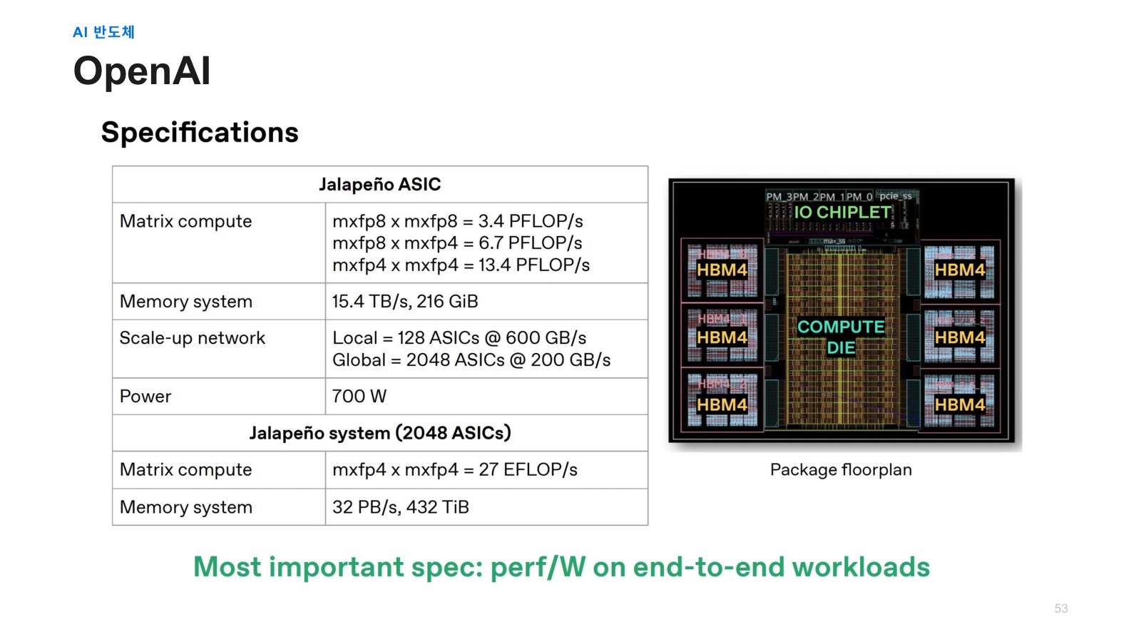
So, to share one recent piece of news, as I mentioned earlier, at a place called Hot Chips, OpenAI unveiled Jalapeño, a very interestingly named AI semiconductor—a proprietary AI semiconductor it developed itself. It also uses HBM4. Even for GPUs using HBM4, it is only with Rubin that NVIDIA is using HBM4. The current Blackwell series all uses HBM3E, so it uses the most advanced memory technology, and one distinctive aspect is that OpenAI’s Jalapeño architecture and the architecture of our product called Bertha, which I introduced earlier, are very similar.
So when we went to Hot Chips to demonstrate it, many people came by and said, “You seem very similar to OpenAI’s architecture,” which we heard quite often. We felt that way a lot as well. To explain a little, there is HBM like this, and we also have DDR alongside it; the data coming from there is handled by the adjacent cores, which receive it directly and perform computations, and the computation results are shared among the cores within it like this, so our architecture and Jalapeño are very similar. I developed it in a completely different place at a different time, yet they could be this similar, which I find interesting.
Chester Roh OpenAI might contact you. Hot Chips is the conference that was recently held at Stanford, right?
Jinwon Lee It is held at Stanford every year. What is interesting is that when you think of a conference, you imagine a very large convention center with multiple separate tracks, right? Hot Chips is a very old conference, but it is held in just one building at Stanford University, in a single space such as an auditorium, without separate tracks, for two days. Major companies in the AI semiconductor industry all attend. That includes NVIDIA, of course, as well as AMD and Intel, and OpenAI participated this time as well. So it is a conference attended by a great many companies.
Jonghyun Park Did you go?
Jinwon Lee I was busy with bring-up, so I could not go, but our CEO and engineers went.
Jonghyun Park I saw on X that at Hot Chips, a gpt-oss 2T-parameter model had allegedly leaked. I saw people saying that.
Jinwon Lee I also only saw that online, so I have not been able to verify it myself.
Jonghyun Park I will take it as a rumor for now.
Prefill and Decode as the Two Stages of LLM Inference 15:01
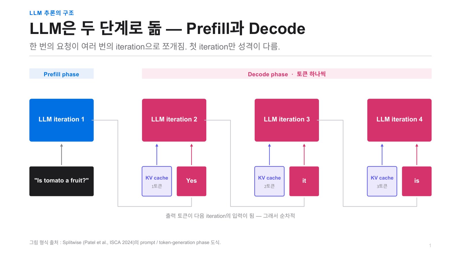
Jinwon Lee Then, let us get started in earnest. First, let us briefly look at how LLM inference works. There is what we call a prompt, which the user provides. When that comes in as input, for example, if the user asks here, “Is tomato a fruit?” then this LLM operates and works hard to compute, then outputs the first token, “Yes.” So, for convenience, let us call this four tokens. Treating one word as a token, when four tokens are provided as input, it computes those four tokens all at once up to the point of outputting the first next token, “Yes.” We call this process prefill.
After that, it works autoregressively, continuing to run, and then when “Yes” comes in as input, the LLM runs another computation and outputs a token called “it,” then “it” goes in and “is” comes out, and when “is” goes in, if what is called the end-of-sentence EOS token, indicating that the sentence has ended, comes out, this iteration ends. So, the part shown in red here, where one token comes in like this and one token comes out next, is called the decode phase. So, the process of LLM inference consists of prefill and decode, divided into these two stages.
Chester Roh With prefill, you mentioned four tokens, but in fact, there could be 1,000 or 2,000 tokens in there, and if we throw in an entire book, it can look through that entire book, but in fact, a GPU can perform this all at once in a single computation, so it makes excellent use of the GPU’s strengths. Since the preceding word has to be processed before the next word can come out, it can only be processed one character at a time then, so this is somewhat slow.
Jinwon Lee This is one of the key points we want to discuss today.
Chester Roh It is divided into prefill and decode. So, in prefill, multiple words go in all at once, and the GPU computes them all at once, whereas outputting them one character at a time afterward is the decode process, and it is highly sequential. Optimizing these two workloads is important in inference, and as for why they take this form, CTO Jinwon Lee is going to teach us step by step. We need to stay sharp and keep up with today’s lesson.
Seungjoon Choi I have a question as well. This also came up when Noah was here, but TTFT, or time to first token, is between the blue and red
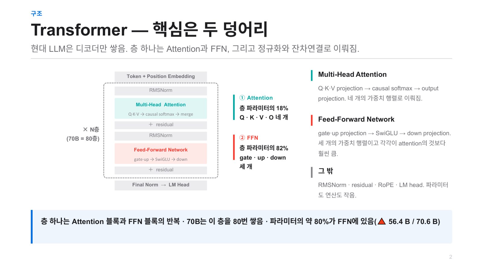
Jinwon Lee That’s right. The time from when this black input comes in to when “Yes” comes out is TTFT, time to first token. Then, when “Yes” goes in and “it” comes out, this one decode iteration is also called TBT, or time between tokens, and TPOT. It is also called time per output token, and there are several slightly different terms. Their meanings differ ever so slightly, but there is no major problem with using them interchangeably. Then, let’s look at what exactly is inside an LLM iteration. There is an algorithm called Transformer in here, and to summarize it once more, the flow goes from top to bottom. When a token first comes in, these days positional embedding is also handled internally, and we use RoPE. That is inside attention, but in any case, when a token comes in, the important thing is the attention I’ve colored, followed by what is called a feed-forward network, or FFN, passing through it, and then repeating this over and over, before finally reaching what is called the LM head to select what the next token will be. But in this model, if we are talking about a 100B-parameter model, that model’s parameters exist, and if we look at what proportion of those parameters are in attention and the feed-forward network, attention accounts for roughly 20%, while FFN accounts for about 80%. So, by about four to one, FFN has more parameters. But this is for dense models, when we are not using the kind of model frequently used these days called MoE. With MoE models, the proportion shifts much more heavily toward FFN. So, there are fewer parameters in attention than you might think. When we think of Transformers, we think attention is the core—and it is. But the most important computations in a Transformer can be considered these two.
Attention and FFN as Transformer’s Core Operations 17:57
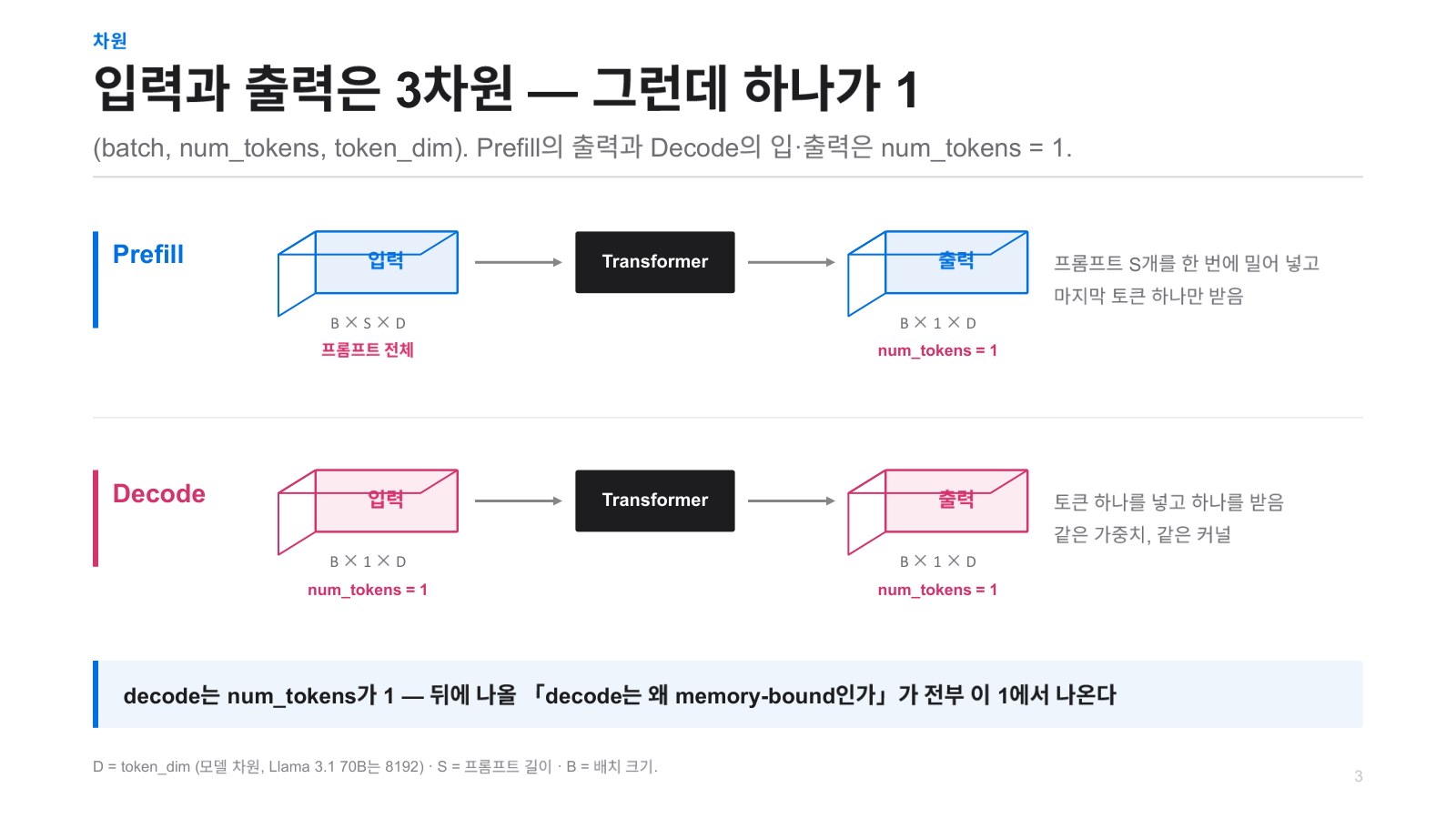
Jinwon Lee So, we will look at that in more detail, but before that, we need to examine the dimensions of what we feed into this Transformer as input and what comes out as output. We need to look at those dimensions. There are three dimensions. The first dimension is batch, which is the batch used when multiple requests come in and are processed simultaneously. Next is the number of tokens. So, when I asked earlier, “Is tomato a fruit?” there were four tokens. Those four tokens, and how many dimensions each token will be represented as a vector, make up the three-dimensional input, and the output is also three-dimensional, but as you saw earlier, in prefill, we do not know how many words or tokens of input a user will provide. It can be up to one million tokens. So, this becomes greater than 1, but because only one token comes out as the result, this becomes 1. So, if we remove this 1, it can effectively be considered two-dimensional. And in decode, one token always comes in and one token comes out, so when we do not consider the batch, data of the same form as the output of this prefill you can think of it as moving around.
Chester Roh The batch we always used in PyTorch, and num_tokens is the sequence length, and the token dimension is the dimension of the Transformer embedding, right?
Seungjoon Choi That’s right. This is a bit confusing. At first, this token is an ID, an integer or a natural number, but from this point on, it’s a vector, right, here?
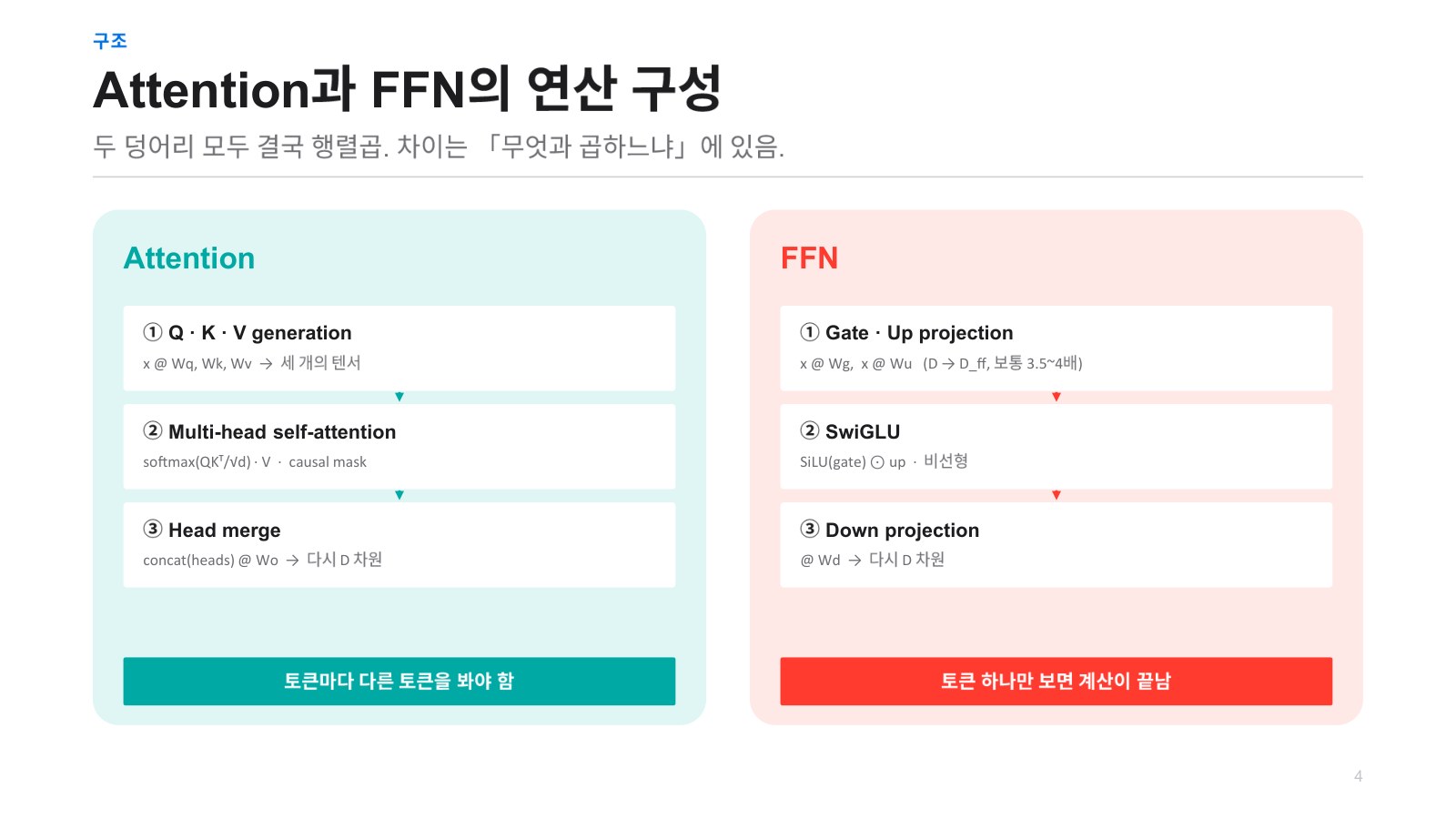
Jinwon Lee That’s where it changes into a vector in the token dimension, where it was originally a scalar and becomes a vector. So if you look inside attention, there are things called Query, Key, and Value, and for each token that came in as input earlier, if the embedding dimension here is 10 dimensions, you represent one word with 10 numbers, or represent one token. You take that token embedding vector and use some weight parameters here, which are model parameters. You multiply each of them and perform matrix operations. That creates Query, Key, and Value. Then a question arises here: the input is three-dimensional, but this is two-dimensional. You may wonder how you multiply them, but simply put, you take B times S and just flatten it. For example, if B here is 5, the sequence is 2, and D is 10, you have 5 times 2 times 10, multiply the first two to get 10, make it into a 10-by-10 matrix, and then think of it as performing the operation. So you multiply this to generate QKV, and then perform operations among Query, Key, and Value. First, you take the dot product of Query and Key, perform matrix multiplication, and then apply something called softmax, then multiply Value again to perform the operation. This is called self-attention.
QKV Operations and the Self-Attention Structure 20:50
Jinwon Lee But you divide this into multiple heads and perform the same operation, so here, you split up all the generated QKV and, if there are 16 heads, divide it into 16 pieces, perform self-attention among those pieces, and later combine them back into one, which is called head merge. So when merging, you concatenate all these results together and multiply them once more by some weight parameter here to produce the result. Then this result goes through several subsequent operations, such as residual connections, and moves on to the FFN. Broadly speaking, the FFN consists of two linear layers. You simply multiply by weights twice. Of course, something called a gate has recently been added, making it a little more complicated, but you can think of it as a neural net with two layers. So the point is that there are many parameters here for computation.
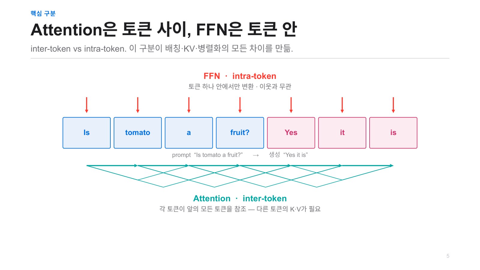
Conceptually, attention turns all of these into Query, Key, and Value, for example, and takes the Query of this one and the Key of these ones, this one’s Key, and computes vector dot products with every Key. That is represented as matrix multiplication, so you can think of attention as learning the relationships between tokens, and when it goes into the FFN, earlier, I said one token could be represented by a certain number of numbers—say, 10, meaning it is represented as a 10-dimensional vector. The 10-dimensional vector consists of numbers, and the FFN performs operations among those numbers. So operations between tokens are attention, while operations among vector dimensions within one token are what you can think of as the FFN.
Coincidentally, if you look back at the CNN era, there was something called depthwise convolution, and it has the exact same form. Once in the spatial direction, it performs operations in the horizontal and vertical directions, and once it performs operations only in the channel direction. So you can think of it as a completely identical structure, and this is where Transformers can be seen as having a somewhat more general architecture.
CNNs have a similar concept called depthwise convolution, but when looking in the spatial direction, they only looked at fixed regions such as 3×3, whereas attention goes from the very first token to the very last token. It does not look ahead, but the last token looks all the way back to the first token and does something, because it looks at everything globally, making it a somewhat more general model. For scalingists like me, it is a more general algorithm that shows performance improves as you increase the scale—a representative example of that.
Jonghyun Park For those watching this, I should mention that matrix operations can be hard to immediately grasp in your head as the dimensions get larger, so if you go to the 3Blue1Brown channel, there are videos that depict this very beautifully with 3D graphics. So if you want to follow what we are discussing now in greater depth, referring to that will be very helpful.
Seungjoon Choi It’s not just that we don’t need to know gates; we don’t actually need to know all of this, right?
Jinwon Lee You can just think, “Oh, something like this exists.”
Chester Roh Yes, actually, this is one step. You need to understand this Transformer paper, how the dimensions inside it work, and even understand the PyTorch code line by line before Transformers naturally start to make sense after that, Before that, no matter how much you examine it conceptually, some things are difficult to understand. That is an unavoidable fact. So regarding that part, just knowing conceptually that there is an attention block, an FFN block, where computation is used heavily, and what these things are will be enough for you to follow the content that comes afterward.
Seungjoon Choi There seems to be something new. I had forgotten about channel-wise.
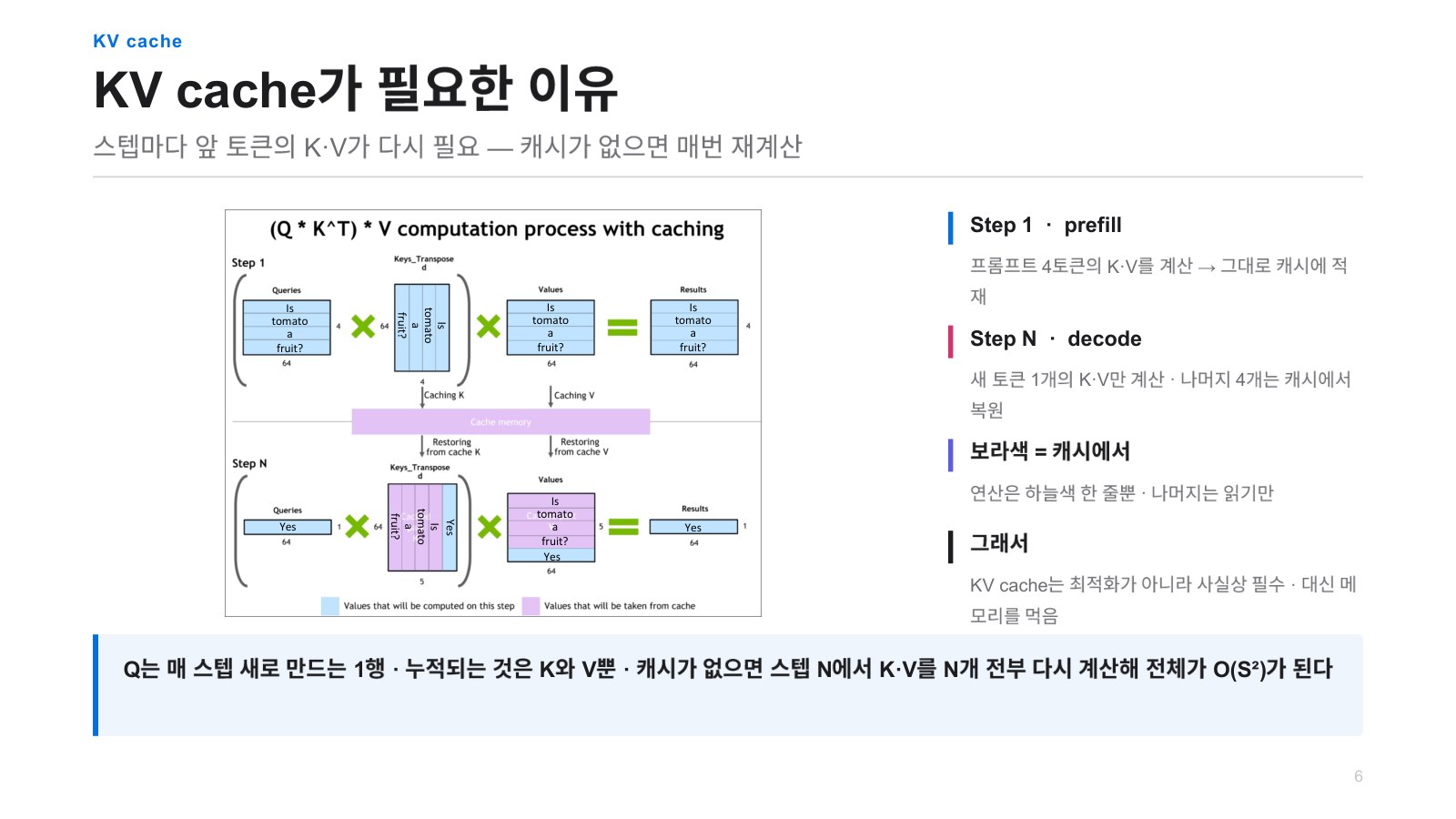
Jinwon Lee So, earlier, if you look closely at the attention part, when there are token embedding vectors, I said that we create Queries, Keys, and Values from them, and when those have been created, this represents the computation process. You multiply the Query and Key, apply something called softmax, and then multiply by the Value again. This happens during prefill, in the example I showed earlier, and with this output, if you perform the LM head operation at the end, the word token ‘yes’ is produced.
KV Cache Reuse of Key and Value During Decode 26:32
Jinwon Lee Then, when we come to the decode phase, ‘yes’ is given as input. Then, using ‘yes,’ we create another Query, Key, and Value, this light-blue section. And for computation, the Key and Value from the preceding tokens are all needed. The Query is not needed, but the Key and Value are. So conceptually, the Key and Value contain the preceding context information. Put simply, when I have a conversation with ChatGPT, the memory of the conversations I had in the past can be thought of as the Key and Value. There are two ways to process this. At this point, the Keys and Values for these tokens can be calculated again, or since they were calculated once here, you could store them in memory and retrieve them later. So, in most cases, storing them in memory and retrieving them later is advantageous, so the Keys and Values generated during the initial prompt phase are stored. Now, with ‘yes,’ when I say that the next token came out here with a single layer, when the next token is entered as input again, ‘yes’ is used again, so the Key and Value for ‘yes’ here must also be stored once this step is finished.
Chester Roh Right. This is what we always call the KV cache. If we brought in a news article from elsewhere earlier and prefilled 2,000 characters, then the KV cache contains all of those preceding 2,000 characters.
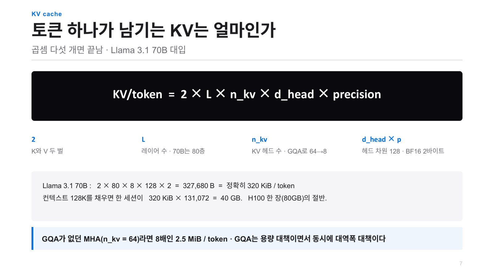
Jinwon Lee We have to retrieve all of that. So the memory space for storing this KV cache needs to be large. So, to find out exactly how much storage is needed per token to store KV, if we calculate it, this uses the Llama 3.1 70B model. The 2 here is multiplied because there are two: Key and Value. So we multiply by 2. N is the number of layers. Since attention must be performed at every layer, it is needed for each layer, and then, for the Key and Value, as mentioned earlier,
KV Cache Capacity Exploding to 320 KB per Token and GQA 28:15
Chester Roh multi-head attention.
Jinwon Lee Multi-head attention is the default, in the transformer algorithm, but Llama 3.1 uses grouped-query attention. What is grouped-query attention? It is labeled GQA here, and for each head, originally there should be one Query, one Key, and one Value, but if, for example, eight heads are grouped together, there are eight Queries for every eight heads, but the Key and Value have only one each, one for every eight, that is how you can think of it. Then you multiply by the number of heads, and determine how many bytes to use to store each Key and Value. Usually, if they are stored in BF16 or FP16, they take 2 bytes. So, if you calculate all of this, it comes to roughly 320 KB, 320 KB per token. So, if we were to store this for a 128K, 128,000-token context as Keys and Values, about 40 GB of capacity is needed. A single H100 has 80 GB of memory, so that is half of it. If one user uses a 128K context, 40 GB of Key and Value storage is needed. And that is with a 70B model. If this goes to a 1T model, it will become enormous.
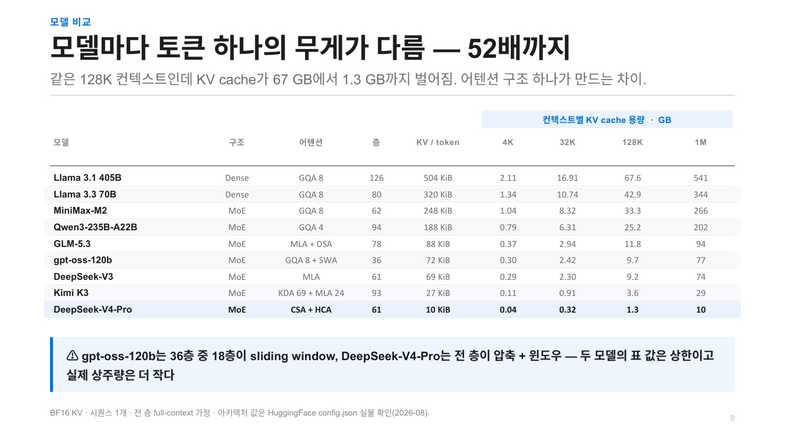
To show that the size of Key and Value storage is larger than you might think, I organized a table of various open-source models showing what attention they use, how much Key and Value capacity they require per token as a result, and how much capacity increases as the context grows. I organized it into a table. If you look here, among the models released recently, Chinese open-source models are a little smaller, as you can see. There are some different types of attention here. So, with this kind of attention, to compress the large amount of Key and Value data generated, various techniques are used to reduce it significantly. If it is not reduced, as you can see here, even compared with the capacity needed to store the model, the memory capacity needed to store Key and Value can become greater. So these kinds of things are happening.
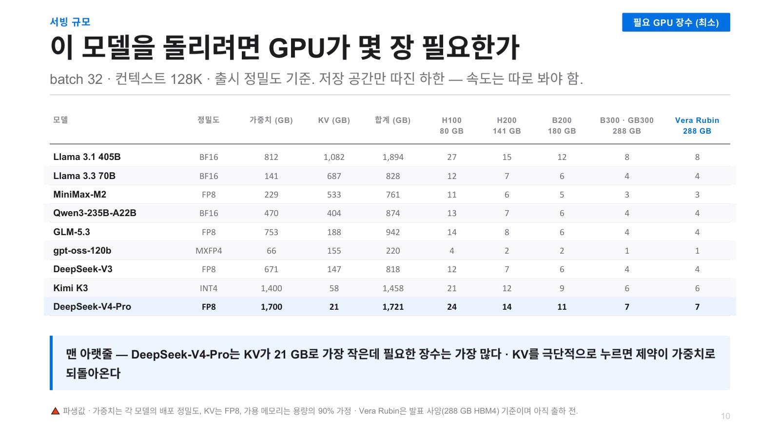
And additionally, to run this, how many GPUs are needed, if the batch is 32—that is, serving 32 people— and the context averages 128K, how much is needed, I’ve listed the required number of GPUs here. In the case of something like an H100, to serve Llama 3.1 405B, 27 are needed. That is only divided by storage capacity, but since in practice you have to use multiples of eight, you would need around 32.
Seungjoon Choi Something I’m a little curious about here is, if you don’t know about things like this it’s fine to use it, but once you use it knowing even roughly about it, this KV cache will disappear over time, and I still haven’t organized my thoughts, so I’m not giving the model any work, but this disappears over time, so in that case, I’d have to do another prefill, and it would cost more—that’s what I start thinking, but there’s no need to think that far, right?
Jinwon Lee Right. If you think about even that,
Exhausting. Leave those things to the engineers who do inference engineering, and use it comfortably.
Jonghyun Park That’s why frontier models, in their pricing plans, instead of subscriptions, if you pay to use the API, they tell you how long they retain that cache, and if the prompt I was using gets a cache hit, is the price about one-tenth? They give you a huge discount. It is a pricing policy made possible by retaining all that KV cache. Regular users do not need to worry about it; they can just assume the cache is all being retained.
Quantization and MLA for Reducing KV Cache 32:12
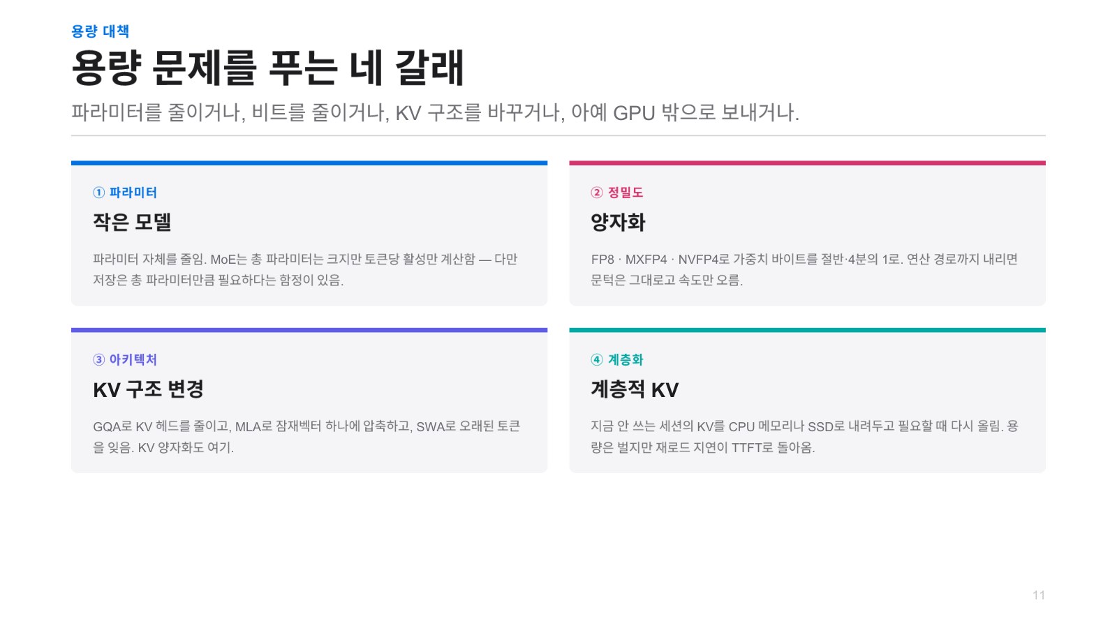
Jinwon Lee Since this capacity becomes a problem, then, to solve the capacity problem, the most intuitive method that comes up is to make the model smaller. Using a smaller model can reduce the capacity somewhat. Next, you can do quantization. So recently, going beyond 8-bit, floating-point formats such as 4-bit MXFP4 and NVFP4, which are not registered in the original standard, have begun to be defined and used by people. Next, as I mentioned earlier, you change the structure of KV. So, with Grouped Query Attention earlier, originally, each head needed its own KV, but if you used one KV for every eight heads, something like MLA, which DeepSeek used, gives just one KV for all queries, and even compresses that into a latent vector to store in memory.
Next, there is something called sliding window attention, which is similar in concept to CNNs. Rather than attending all the way to the very first token, it attends only to a few tokens around it, with a defined window size. But using only this can somewhat reduce performance, so it is usually used as a hybrid. One time, it looks at everything, and another time, it uses a sliding window.
Next, since there is not enough space to store KV, systems like Mooncake move it to CPU memory or offload it to an SSD, then bring it back when needed and use it— that approach is discussed a lot. As agentic AI has emerged, the amount of KV being generated is now, compared with earlier reasoning models, at a level that cannot even be compared, so there is no way to keep it all in memory, and as I’ll mention later, people set it running, go do something else, and because the agent takes a long time, come back and say, “It’s all done.” During that period, the server cannot keep storing KV in expensive HBM memory, so methods that move it to other memory like this are also widely used.
Seungjoon Choi When using an inference-specific chip, even if architectures that handle KV in this way keep changing, can already fabricated semiconductors handle it all?
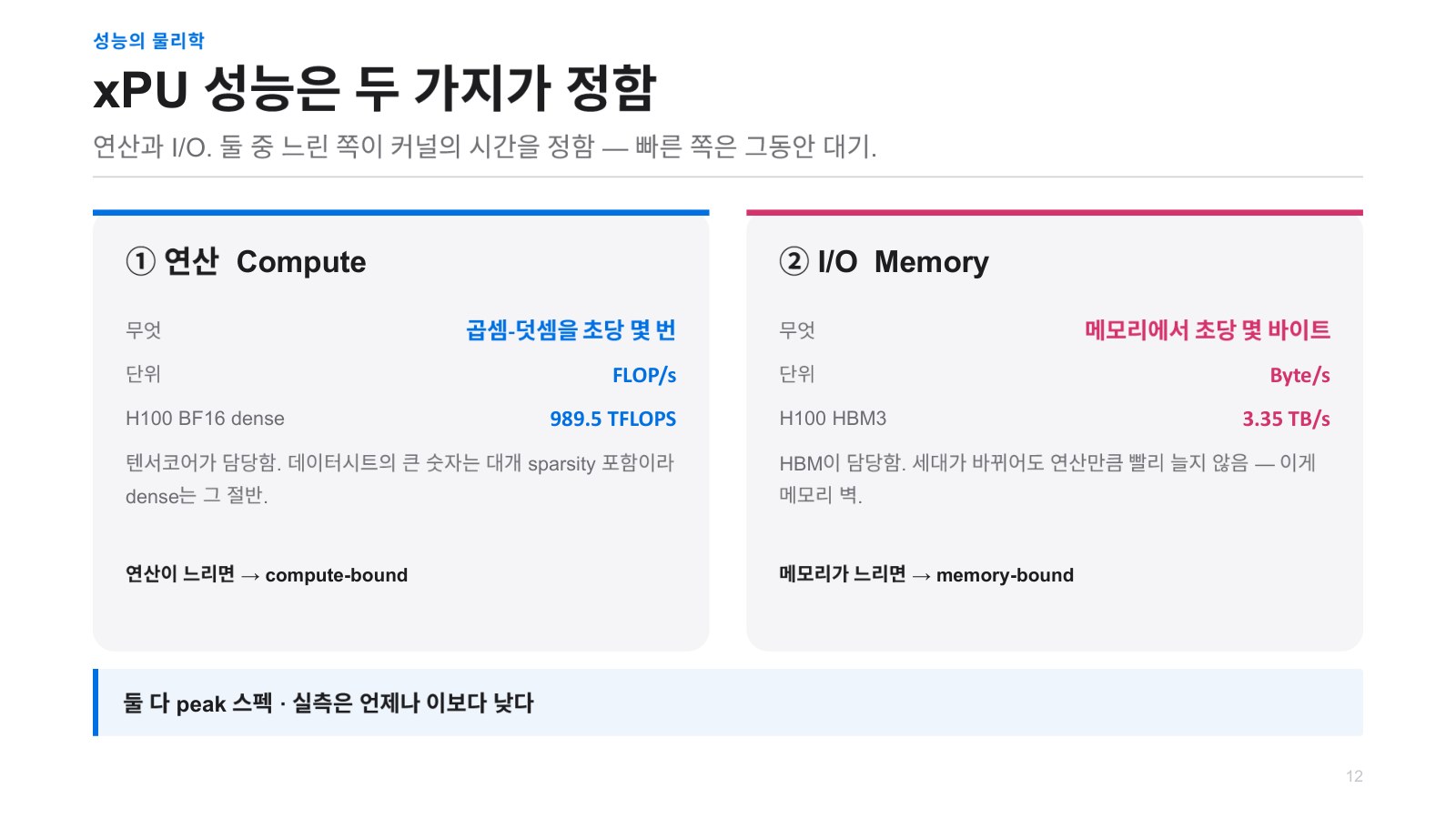
Jinwon Lee That can vary depending on the situation. So usually, it is quite possible that it was not taken into consideration. Because in the past, people likely did not think much that space would become this abundant. But newly emerging ones are being designed with considerable consideration for using such things. Next, moving beyond the discussion of capacity, whether it is a CPU or GPU, which is why I called it an XPU, what determines XPU performance is, simply put, two things. When adding A and B in some computation, both A and B are initially in memory. So after reading A and reading B, adding the results and calling that C, and then storing that C back in memory, if there is such a simple operation, there is the need to read data from memory and then the need to perform computation, and depending on which of these two is faster, performance encounters a bottleneck on one side. The reason is that the example I just gave reads A and B, performs the computation, and stores the result in memory, which I explained as a serialized operation, In reality, it doesn’t work like this; it reads A and B, and while it is adding A and B, it is also reading C and D for the next operation. That way, as soon as this operation finishes, it can add the next C and D as well. In AI, processing has to be done in parallel, and because the same operation has to be performed an enormous number of times, this naturally happens. Whether it’s a GPU or an NPU, how many operations they can perform per second, and how quickly they can supply data from memory, these two factors determine where bottlenecks occur.
Distinguishing Compute Bottlenecks from Memory Bottlenecks 35:01
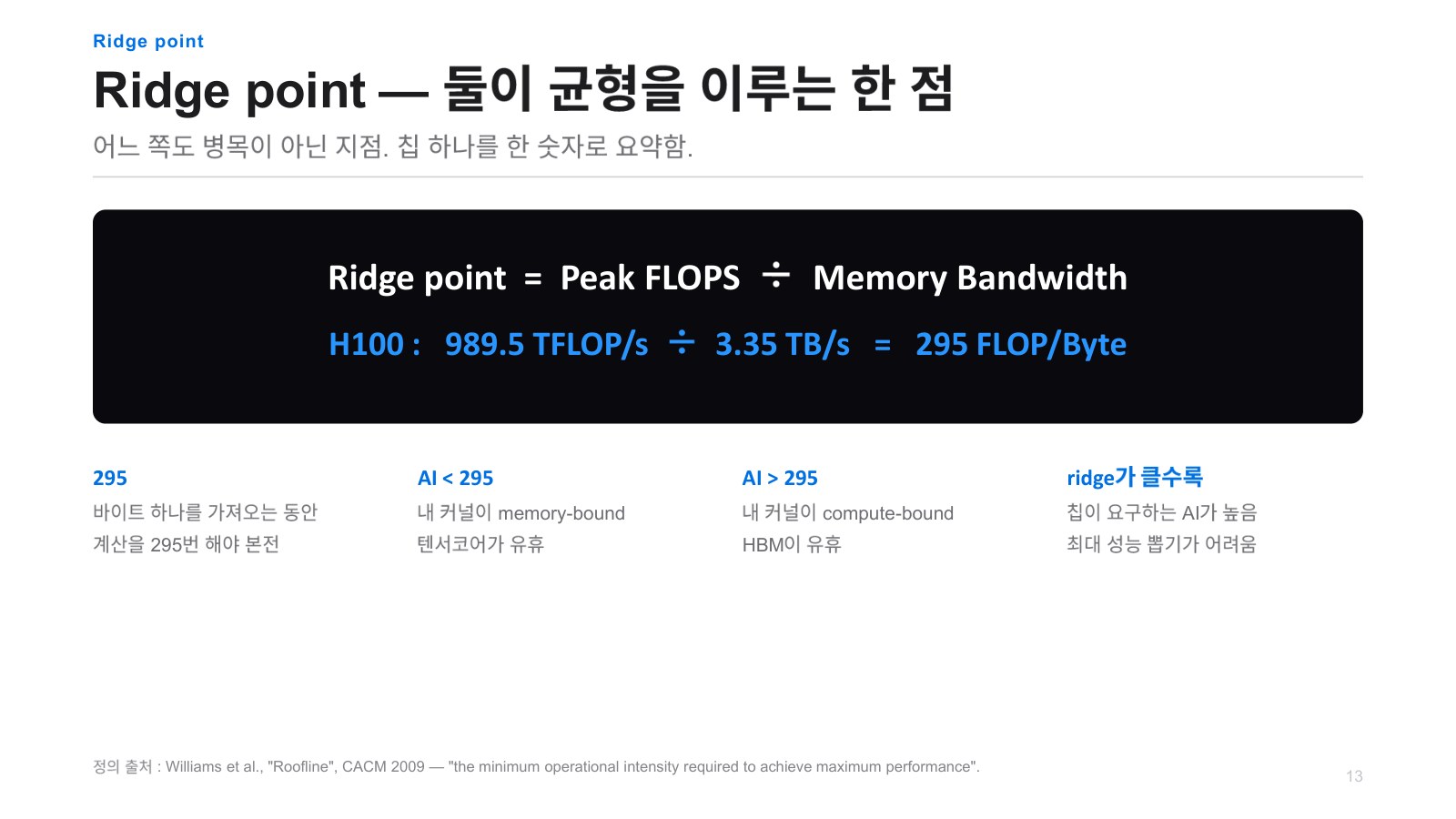
Jinwon Lee Usually, compared to the data being read, they are designed to perform far more computations. For example, if you look at something like the H100, based on BF16, or 16-bit data, it can perform about 1 PFLOP/s of computation. That’s about 1,000 TFLOP/s, while what it reads from memory is 3.35 TB per second. Then, if this is actually BF16, the number of data elements would be half that amount. Because each data element is 2 bytes. So if you roughly calculate this ratio, simply dividing gives you 300. So the point at which the two are exactly balanced, where neither computation nor memory is slower or faster, if you calculate the point at which they are balanced, it is roughly 300. This is called the ridge point. For example, suppose this is a hardware metric, and I run a certain AI model, and the program called a kernel that runs that model reads data from memory once, but can perform only 200 operations. Then the bottleneck will be on the memory side, whereas this model, when it reads data once, can perform 1,000 operations. Then it reads the data once and tries to perform 1,000 operations, but it can currently perform only 300 operations. So even though it could run faster, there are not enough compute units. In this case, it becomes compute-bound.
Definition of Arithmetic Intensity and Data Reuse 37:48
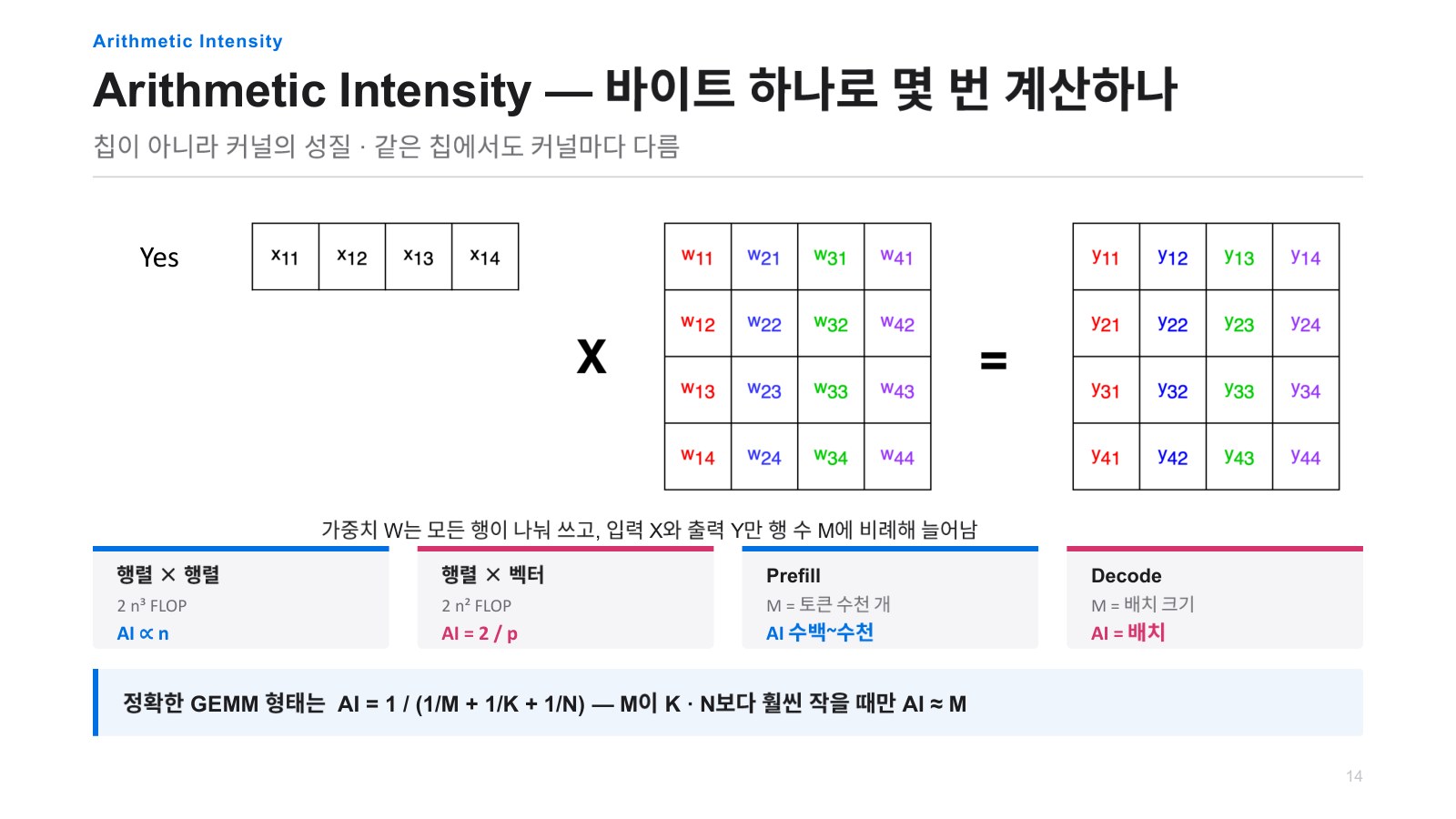
Jinwon Lee So this AI does not mean Artificial Intelligence, but Arithmetic Intensity, or arithmetic intensity, when reading 1 byte of data from memory, refers to how many operations can be performed on it. This may be a somewhat difficult concept, but I’ll explain it with an example. Earlier, the four tokens from the question, “Is a tomato a fruit?” were represented as four-dimensional vectors. You would multiply them by some weight and perform many such operations. You would perform these operations when generating a query as well, and you would also perform them in the FFN, although the matrix sizes would differ somewhat. To explain it simply, I represented it as a 4×4 matrix. Then, from the perspective of this weight parameter, if you look at how many times this W11 is used in multiplication, it would be used four times. It would be multiplied by this as well, and by that as well, so this data, W11, when you read one of it, if you ask how many operations you can perform at most, you can perform four. That is Arithmetic Intensity. More precisely, in AI semiconductors or GPUs, every multiplication is followed by one addition. Because here, this vector and this vector are being multiplied in a dot product, you have to add up all these results. Multiplication and addition always occur together as a pair, so they are counted as two operations, but whether it is one or two is not important; the order is what matters here.
Ultimately, if you look at what this Arithmetic Intensity is affected by, it is affected by the number of tokens. And as I said at the very beginning, this number of tokens is originally three-dimensional in the input, but when entering as input, batch times token sequence length are combined into one. So if data from other batches are also stacked below, that is included as well. So it would have an Arithmetic Intensity equal to batch times sequence length. For example, let’s simply assume the batch is 1, and suppose you use one million tokens. Then the Arithmetic Intensity becomes one million. Conversely, when it comes to decoding, this is just one. So what is called W11 is used only once. So at that point, the Arithmetic Intensity is 1. And this thing called Arithmetic Intensity is a slightly different topic, but it is extremely important in semiconductors. Because reading data once from memory and performing many operations means making extensive use of it. Conversely, for the same amount of computation, it means the number of memory reads decreases.
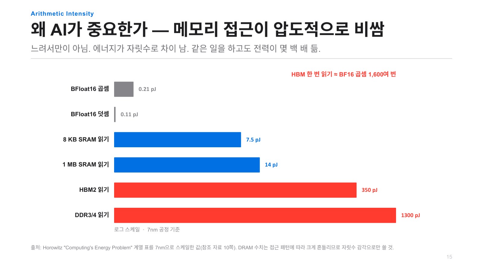
The reason this is important is that, if you look here, compared to the energy consumed by one multiplication and one addition, this SRAM is memory that is even inside the chip, but when reading from SRAM, HBM, or DDR, if you look at the energy consumed, how many orders of magnitude apart are they? They differ enormously—by as much as four or five orders of magnitude. Because they consume so much energy, when we talk about low power, the most important thing is how little data we read from and write to memory, This is extremely important. And that is also connected to Arithmetic Intensity. That was a slightly different topic. So, Roofline analysis emerged, and it is a well-known paper published by several people, including David Patterson, in 2009. What I referred to earlier as the ridge point is a line that is drawn once the hardware is determined. It is not a line related to any particular model, but rather a graph that represents the performance of the hardware. This ridge point is a state with no bottleneck in either compute or memory.
Reading Compute-Bound and Memory-Bound Through Roofline Analysis 40:58
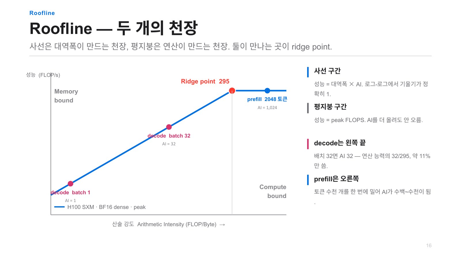
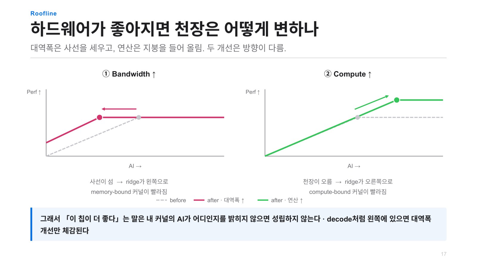
Jinwon Lee The way to draw this is, this flat line here represents the maximum computing capability a semiconductor can deliver. Earlier, I said that an H100 can perform about 1PFLOPS of computation, and that is this point here. If you follow the y-axis here, you get about 1,000 TFLOPS on the y-axis. Then, this slope has a slope of 1 when plotted on a log-log scale, and the point corresponding to the y-intercept, where it meets the y-axis, is the bandwidth. Because this slope is always 1, as bandwidth increases, this slope will rise. Then the ridge point will move to the left. Because data is supplied faster, the ridge point forms at a point with lower arithmetic intensity. Conversely, if bandwidth stays the same and compute increases, this horizontal line moves upward, so it goes up like this.
So, what can we learn from this graph? If it is to the right of the ridge point, it is compute-bound. The x-axis is arithmetic intensity. When running a model, as I mentioned earlier, you load the weights during prefill, and can perform one million operations with these weights. Then, since this point is 295, one million would be far to the right. In other words, you can read the data once and perform one million operations, but the compute unit can only perform 300 operations at a time. So it has to perform this multiple times in batches of 300 and wait until it reaches one million operations, which is why it is compute-bound. Conversely, if you move to the left, during decode, you read data from memory and can perform only one operation. But the data from memory arrives at one three-hundredth the speed. So, by that much, performance drops dramatically.
So for prefill, we can still increase the number of compute units if we want to, but in decode, the operation itself is fundamentally structured so that one token goes in and one comes out, and because it is not matrix-by-matrix multiplication, but vector-by-matrix multiplication, arithmetic intensity inevitably ends up at a very low point. So we need to move this to the right, because the point where this graph meets in the y-axis direction ultimately represents performance. The idea is to somehow move this to the right. That’s the thinking. The easiest way is to increase the batch size. Even during decode, one word, one token, from the answer to my question, one answer token for the second user, the third user, the fourth user, if you gather together the output tokens from multiple users and multiply the matrices, arithmetic intensity will increase accordingly. Earlier, I said the input was three-dimensional and that the sequence length was 1. During decode, if you increase the batch size, you can make it two-dimensional again, thereby increasing arithmetic intensity. So during decode, we try to make the most of batching for processing.
Improving Decode Efficiency with Batching and the Limits of Attention 43:46

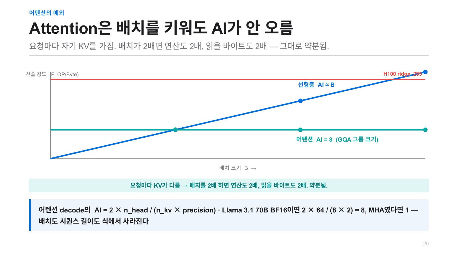
Jinwon Lee But a very serious problem arises here: even if you increase batching in attention, arithmetic intensity does not increase. The reason is, the key-value for my question and that for another person’s question are different. So when you multiply query and key, the query is a vector and the key is a matrix, but you cannot share that matrix. When generating queries, keys, or values across batches, you multiply by the same weights, so you could gather tokens from different users and compute them together, but if this is the query for my output token, and this is the collection of key-values, another user cannot use these key-values. So this is a place where you can never increase arithmetic intensity. It has to remain at 1 here. So attention creates many bottlenecks. Especially recently, as context length has increased, this part has become a very large bottleneck.
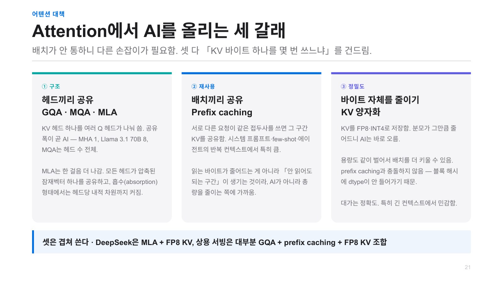
So people would not just sit still. The idea is to increase arithmetic intensity in attention as well. If you use something like the GQA mentioned earlier, there is one key-value for every eight, so you gather eight queries and multiply them by the key matrix, giving you arithmetic intensity of 8. It increases from the original 1 to 8. MQA is also called multi-query attention, and if there are 16 queries, then across all 16 of them, only one key and one value are used. MLA is the same, except MLA compresses even those keys and values. So in such cases, depending on how many queries are assigned one key-value pair, arithmetic intensity increases accordingly. Next, when we give a prompt to ChatGPT or Claude, we cannot see it, but before it, there is a system prompt, information about various tools, and things like precautions included. The part that comes before it is always the same, so the key-values for the hidden prompt are calculated in advance, and sharing and using them is the prefix caching method. This gives us some benefit in that part. And if we reduce the size of the key-values themselves, with the same bandwidth, we can read in more key-values, so that would also be effective. So one method we use is to quantize key-values to 8-bit or 4-bit before bringing them in, and these kinds of techniques are also used in attention as a way to increase arithmetic intensity.
Jonghyun Park So that listeners can understand this more easily, I’d like to explain it in simpler terms just once. Arithmetic intensity refers to how many computations we perform after reading data from memory. If we reuse it as much as possible, the more we do so, the more compute-bound it becomes, so we can make use of the GPU’s computing resources, which are called CUDA cores. Since there are many cores, we can utilize them, so in the case of prefill, we perform calculations on the fetched weights for all tokens at once, making it compute-bound, whereas decode can go the other way because fundamentally, a Transformer has to compute one token at a time, so it cannot reuse them and becomes memory-bound. So, in order to improve the hardware’s own performance, to raise the y-intercept on the next page, and to better handle memory-bound workloads, we use memory with high bandwidth such as HBM, change that curve, and make it as efficient as possible. That’s how I understand it.
Jinwon Lee That’s right. The farther left this goes, the more easily it becomes compute-bound. So we can get better performance out of it.
Chester Roh This ridge point, this curve itself, has nothing to do with the Transformer. Once the hardware is determined, because of compute and memory, it is an optimal line that emerges, and within that optimal line, we have to force the Transformer in. But because prefill and decode in a Transformer have such fundamentally different computational characteristics, the question is how to optimize and fit it in in order to get as much performance as possible from that hardware. Those are the optimization topics we will discuss going forward, right?
And before moving on, let me offer everyone some reassurance once again: It’s okay if these things do not immediately stick in your mind. You do not need to understand all of this, as long as you take it as the framework of thinking that arises to interpret these things within the economics of inference, and as the frontier of engineering. That’s enough.
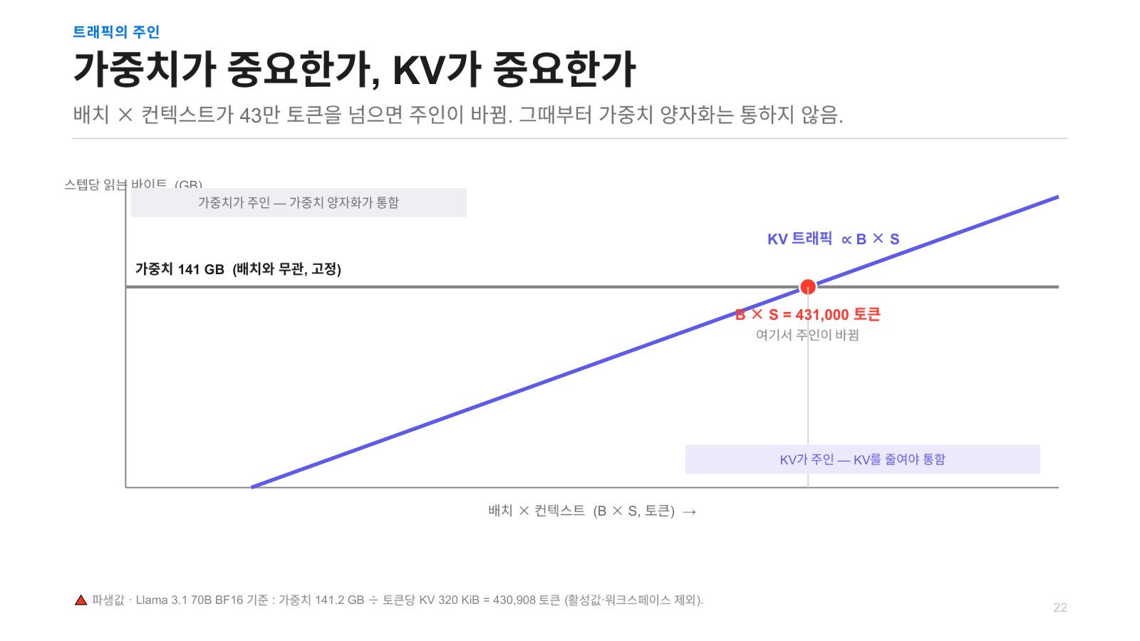
Jinwon Lee So the next thing to discuss is, for example, if we apply some kind of quantization to use memory space a bit more efficiently and, with the same bandwidth, want to read more data, then to see what is effective to quantize, it inevitably relates to which data has a larger volume. We have to go back to the earlier discussion of capacity, and this too, earlier, for Llama 3.1 70B, using BF16 as the basis, the weights are roughly 141 GB, that is about how much the weights occupy, but the point at which key-values become larger is when we use 431,000 tokens. At that point, the key-values become larger. This is based on batch size 1. As the batch size increases, batch multiplied by sequence length corresponds to the arithmetic intensity mentioned earlier, and key-values are generated accordingly, so as the batch size increases, naturally, the amount of key-values reaches a point where it surpasses the amount of weights with fewer and fewer tokens.
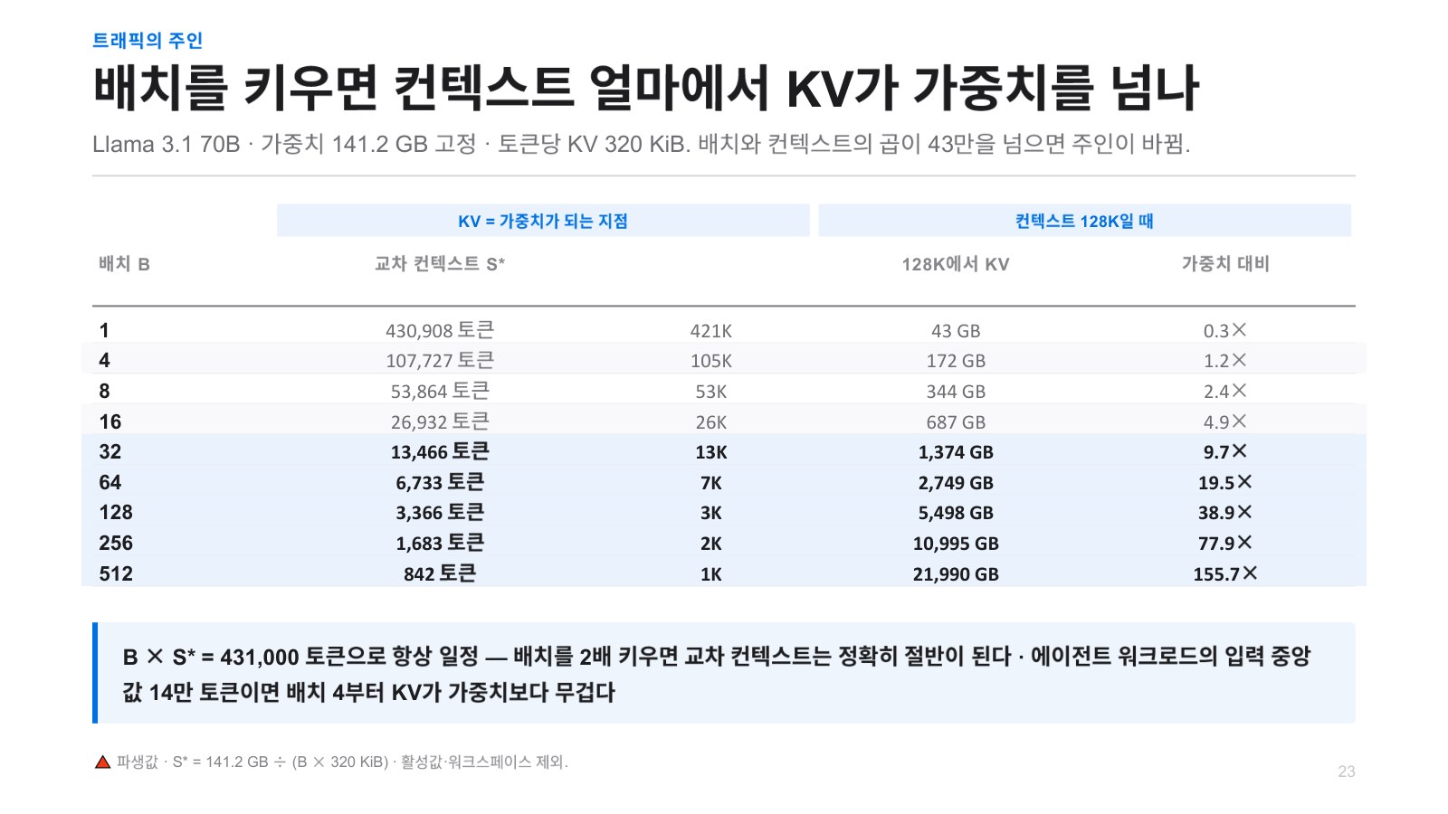
And this calculates how large the key-values are at 128K, and as you can see, at a batch size of 512, it is about 22 TB. So in practice, serving 512 people simultaneously on one server or one or two servers is impossible, as you can see here. So this is meant to show that the amount is large.
Chester Roh Here, B multiplied by S, This is a very important number that determines prefill’s arithmetic intensity, after all. But this batch is something people studying Transformers often get confused about: the concept of a batch when training a Transformer and the concept of a batch in inference are somewhat different. When training, a batch refers to how many sentences we feed in here at once, but in inference, because sequence lengths vary so widely, this batch is the number of users— if you think of it as the number of people using it, that is exactly right. I think this is something you should not confuse.
The Trade-Off Between Interactivity and Throughput 51:33
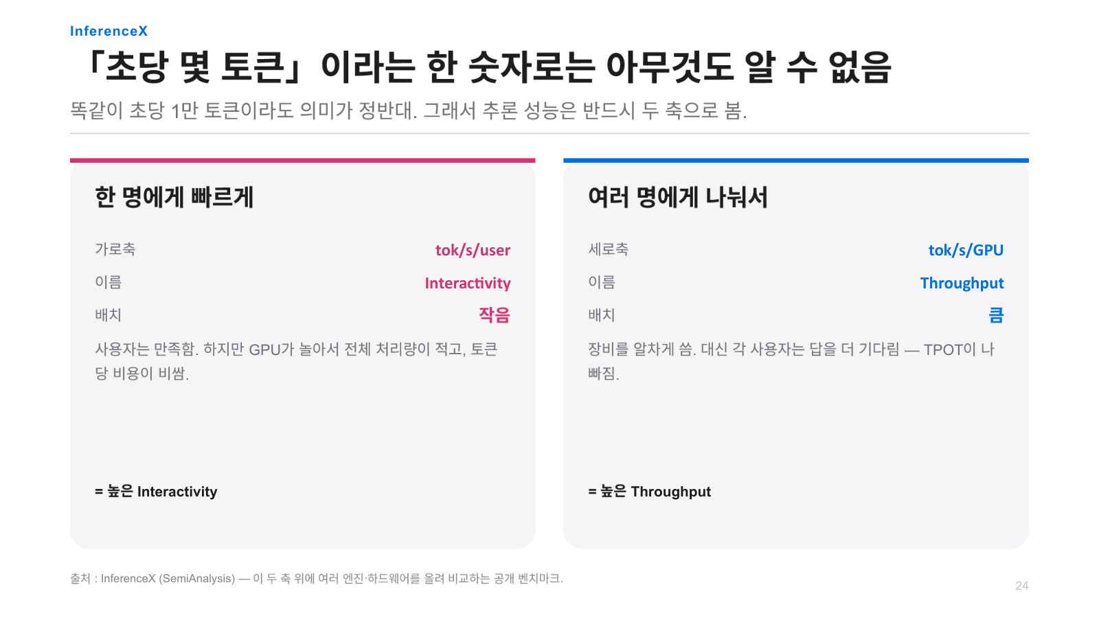
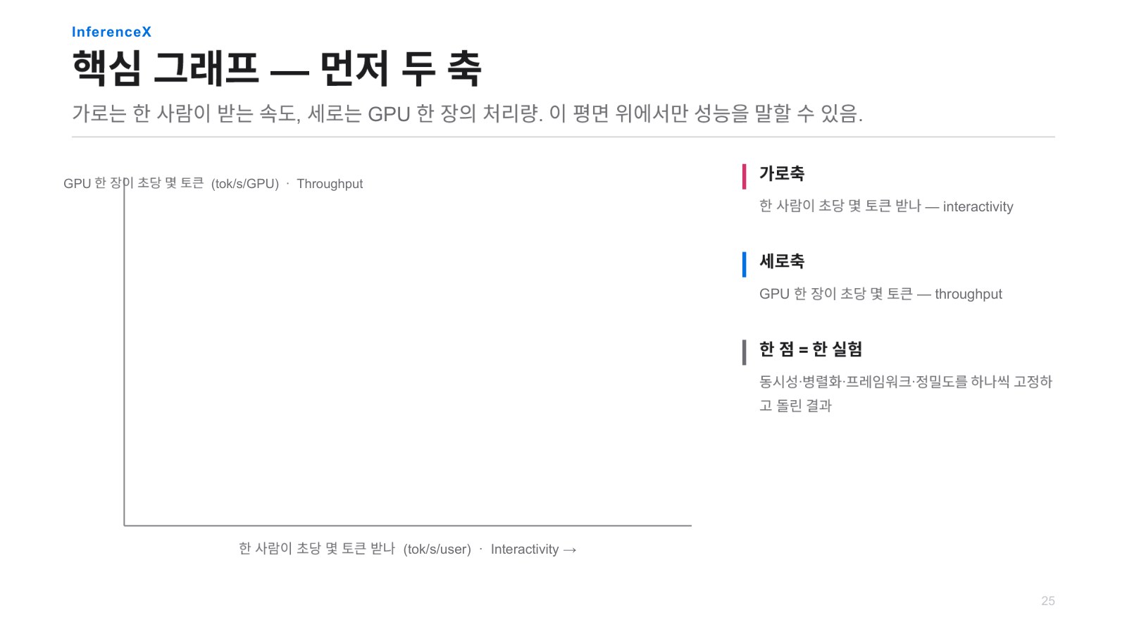
Jinwon Lee That’s right. And I’d like to talk a bit about benchmarks. So which AI semiconductor, or which GPU, is actually good? We also hear that question a lot: “How good is yours?” But it is very difficult to boil this down to a single number and say, “We’re this many percent better than anyone else.” It is very difficult to put it that way. That is because the conditions are so diverse. So a representative metric is how quickly a single user receives tokens, tokens per second per user. How many tokens are delivered per second— that is called interactivity. And from the server’s perspective, I am serving multiple people right now, so the sum of all the tokens being served to those people, divided by the number of GPUs— how many tokens per second each GPU is generating, regardless of whether they are going to one user or 100 users, adding them all together— is called throughput.
Even this morning, when I was going to record this, I was hungry on my way to the office, so I went to McDonald’s and ordered a McMorning, and even though I could see them making it inside, it did not come out even after I waited quite a while. When I looked, they were putting down buns for several people’s orders one by one, bam bam bam. That increases throughput, and I was the first person to order. So my interactivity ended up being in a very bad state. So what I want to say now is that when you increase throughput, you inevitably have to sacrifice interactivity to some extent, and when I happened to see that this morning, it immediately made me think of this.
Jonghyun Park I think this was the point mentioned in the previous episode with CEO Noah, that in order to keep increasing the token speed for one person, you have to sacrifice something else.
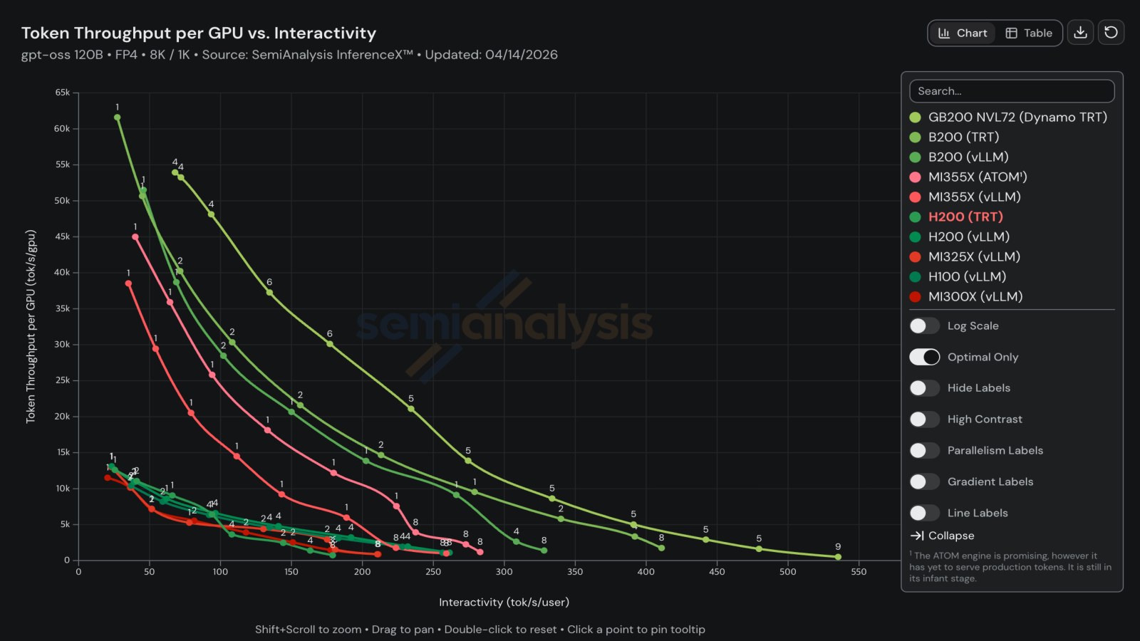
Jinwon Lee And most frontier labs now, when they provide services, have things like fast mode. For example, Anthropic is 2.5 times faster but charges six times as much, and this is where that comes from. To provide faster service to a single user, throughput decreases, so they have to charge more. So this is a benchmark graph created by SemiAnalysis. It does not come out as a single number, but as a graph: the x-axis is interactivity, and the farther right you go, the faster it is. Users receive more tokens per second, and the y-axis is throughput. So depending on a wide variety of circumstances, how many metrics you divide this into, there is tensor parallelism, expert parallelism, pipeline parallelism, data parallelism, and various other techniques, and with all of those as different options, varying everything by batch size, if you plot each point one by one, you end up with a great many points like this. Among these points, the darker-shaded ones at the top right are connected to one another, and when you draw the Pareto curve, it looks like this. This is the core graph of InferenceX. You can never go above this curve, and as you move to the right, the batch size decreases, reducing the number of people being served simultaneously, so speed increases; as you move left, from the server’s perspective, or the GPU’s perspective, it generates more tokens, but each individual user becomes slower.
How to Read the SemiAnalysis InferenceX Pareto Curve 54:26

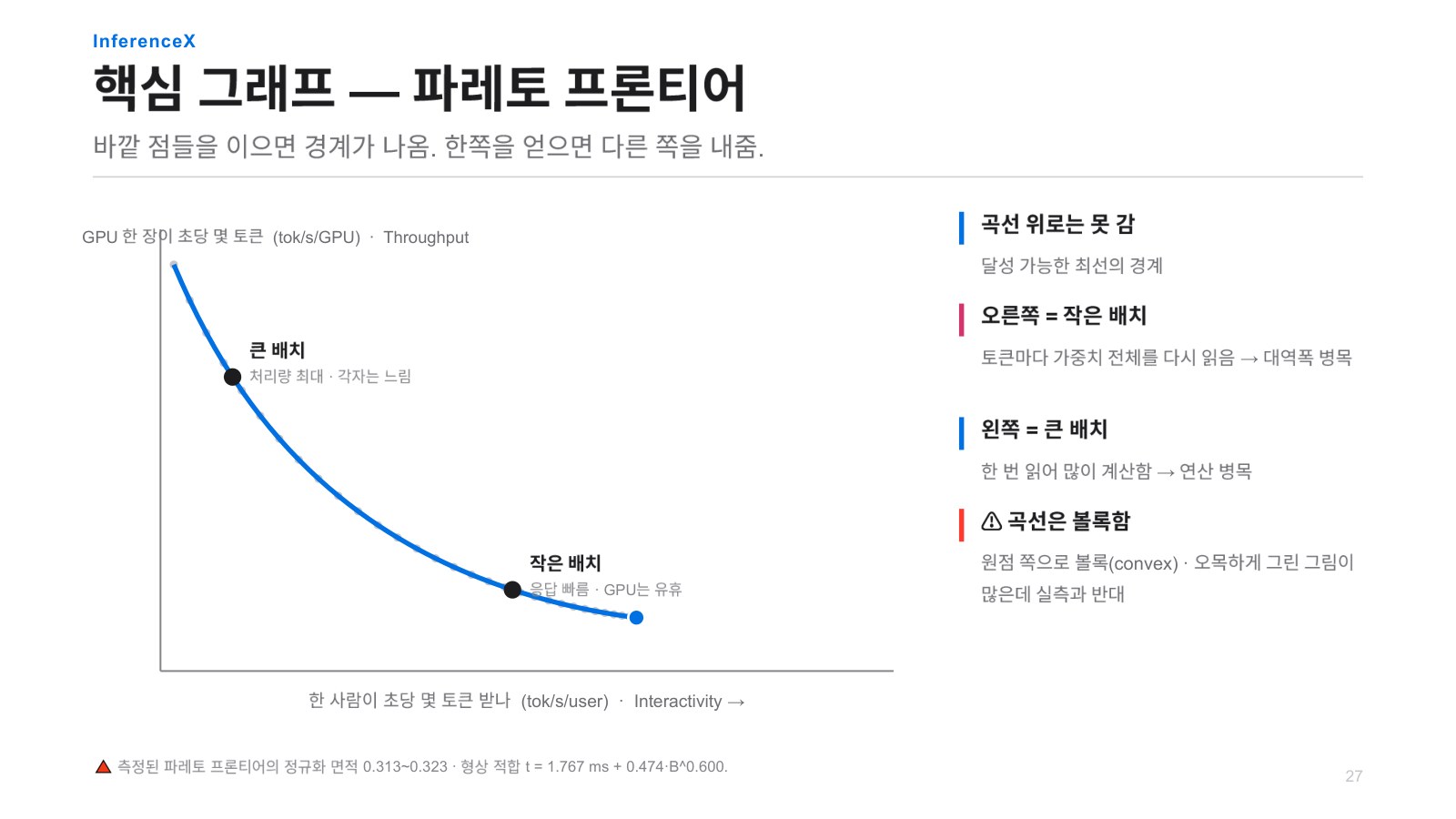
Jinwon Lee If you think about this intuitively, I said earlier that as the number of users increases, the KV cache keeps growing by that amount. So when serving only one user, you only need to read that one user’s KV cache, but if you serve 10 users, you also have to read 10 times as much KV cache data, then perform attention with it for all 10 users before moving on to the next layer, and if there are 100 layers, you have to repeat that 100 times, because reading the KV cache takes longer as the number of users increases. And I said the KV cache is large. Because of that, a single user inevitably experiences slower speed. So that is the conceptual way to think about it. If I show you the actual graph, it looks like this. On the right, you can see the various GPUs, NVIDIA and AMD GPUs. The ones on the left have high throughput, and user interactivity is low, and you can think of the right side as being fast.
Seungjoon Choi When we drew the Pareto frontier graph earlier, were we assuming a single GPU, whereas here we are using multiple GPUs?
Chester Roh We just plotted what the curve looks like for each GPU.
Seungjoon Choi So the earlier one assumed a single GPU,
Jinwon Lee No, it uses multiple GPUs, but here we divide by the number of GPUs. So even if we use 100 GPUs, we divide by 100, which makes them all comparable on the same axes here.
Seungjoon Choi I mean, are you making a plot using one brand, or rather, one product?
Jinwon Lee This is where all of those are collected. So in fact, for even a single graph like this to come out, you need a great many experiments.
Chester Roh So this is essentially different depending on what hardware you use, different depending on what model you use, and also depending on what inference orchestration software you use, and you can see all of those criteria here at once.
Jinwon Lee So if you go to the actual site and hover your mouse here, it shows what configuration it is, including all the software. There is a rough indication here as well, but it differs depending on whether you used vLLM or something like SGLang. It also differs depending on how you set up parallelism, so how do you compare this? Usually, if there is a service, that service has defined requirements, and if we say users absolutely have to receive at least 100 tokens per second, you draw a vertical line at the 100-token point here and compare throughput to see which one has better performance. You can see it there. In this graph, the curves mostly do not intersect, but when you actually plot them, there are quite a few cases where they do. So in regions with good throughput, where the batch size is large, some perform poorly, but as you move to regions with smaller batch sizes, you often see them rise upward like this. So it depends on the situation, but coincidentally, in this graph, what performs well on the right always performs well on the left too, but the behavior on the right and the left can vary depending on the characteristics of the hardware or software—that is what I want to point out.
Seungjoon Choi Then who is this graph useful for?
Chester Roh For businesses that need to take an actual model and build a service to serve it, depending on which stack they choose, this determines whether they make money or not. Because what is missing here is how much they will charge users,
Jinwon Lee That is actually included in a single configuration within this point. Something called disaggregation, which I will discuss later, also makes a huge difference depending on whether you use it or not.
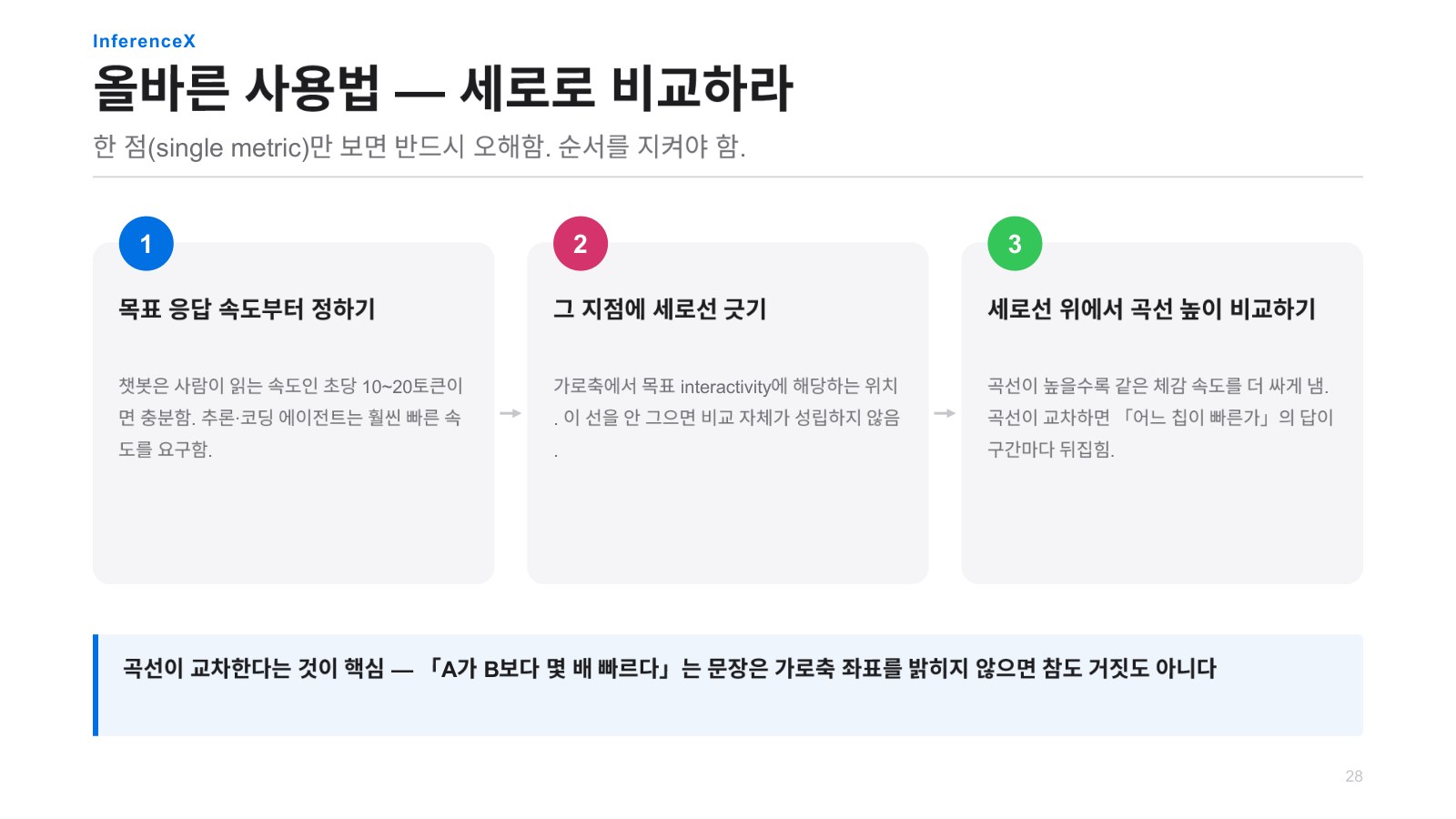
Jonghyun Park Once the user’s required token count and interactivity are defined, when I buy a particular GPU, I can see how much throughput it delivers, meet demand, and calculate how much I could earn or how long it would take to recoup the investment; I think this could be sufficiently useful for modeling as well.
Chester Roh That is exactly why SemiAnalysis does this, I suppose. So, for example, ChatGPT or Anthropic buys certain machines and builds a certain cloud, then charges users a certain amount, and whether they are making money or losing money— by looking at this graph, you could roughly work all of that out in reverse.
Jinwon Lee So they use this to estimate those companies’ revenue as well, and by using an enormous amount of data, SemiAnalysis sells that kind of information as a business that generates revenue.
Chester Roh Anthropic’s token margin being 70 to 80% was probably reverse-engineered based on this kind of analysis as well.
Jinwon Lee And if you look at this year’s GTC as well, Jensen Huang showed how things improve when using something like an LPU, all through this graph. When moving to the right here, it does not drop this much and stays steady. If you use an LPU, because the bandwidth is extremely good, on the side with smaller batches like this, it can deliver good performance. There are examples that show this, and if you understand the concept to the extent of, “Oh, I see,” then even when you see a graph like that, you will think, “Oh, this is what it means.” I think you will be able to understand it.
Seungjoon Choi It seems SemiAnalysis’s standing has changed dramatically. It is being cited everywhere now.
Jinwon Lee Yes, it has changed dramatically.
Chester Roh The company is already enormously profitable. It has never taken investment, and these reports, on what the economics of frontier labs look like, and what kind of curve these companies will reach within two or three years relative to their investment, are being sold as reports to companies around the world, and there are a great many people who want to know. We are curious about it ourselves, so wouldn’t these enormous corporations be even more curious? So I understand that they are gladly paying a great deal of money for it.
Jinwon Lee When we went to ICML at the time, we met with them once, and after that, we also had several meetings online.
Chester Roh AI Frontier and SemiAnalysis held a party during ICML last July. At Lablup. At that time, many chip companies in Korea and large corporations, and SemiAnalysis, we once arranged an exchange between them.
vLLM’s Continuous Batching and PagedAttention 60:51
Jinwon Lee And I’d like to explain some of the features of vLLM for serving. In practice, users’ requests will come in continuously, right? They do not all gather together and arrive at once with a bang; they will come in very randomly, so at the server, in the data center, how to accept and serve them is extremely important. That is why serving frameworks like vLLM and SGLang have become very well-known, and even though they are open source, people use them almost like a standard.
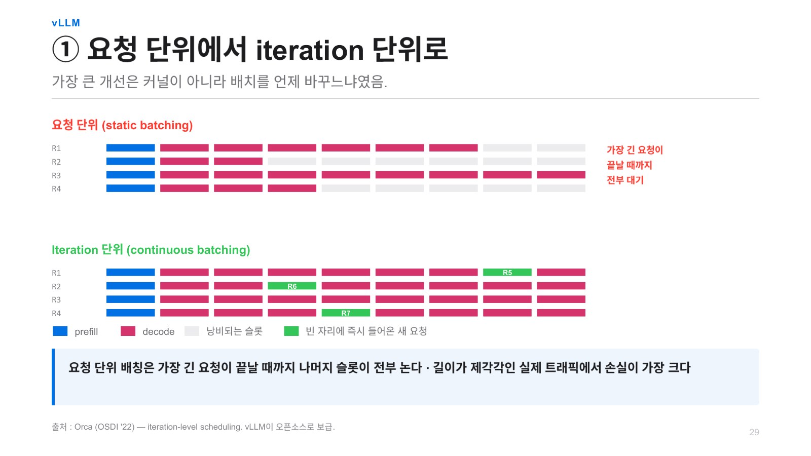
So in the past, people thought of it simply: suppose, for example, that four requests came in simultaneously. If the blue part in front is prefill and this red part is decode, grouping these together into a batch is called static batching, and with static batching, until this batch is completely finished, until all four are finished, the next request cannot come in. Then, naturally, everyone ends up waiting for the longest one.
But then this lighter-colored portion is wasted, so to prevent that, although it did not first start with vLLM, there is something called Orca here, a paper from Professor Byung-Gon Chun’s lab at Seoul National University, and he has also founded a company called FriendliAI, and what it proposed was not to do this by request, but by iteration. What that means is, every time one token is generated, we reschedule. So, after prefill finishes, we take a look once, then after generating one token in decode, we take another look, because these are all generated simultaneously. So when generation has reached this point, the second request, called R2, has finished. Then, in the next iteration, it takes the next item in the queue, called R6 here, and accepts it. So it performs prefill, and at a given step, prefill and decode are mixed together. You can think of green as prefill. This lets you keep it fully packed.
But how do you do prefill and decode together? You might wonder that, but if you think carefully, generating queries, keys, and values, and the FFN all involve multiplying by the exact same weights, so there is no difference at all between prefill and decode. The only difference is attention. In other words, depending on the batch, attention has to be handled separately, so as long as you can separate just that, there is no problem processing them together. In fact, even in this decode step, among these four batches, or in this prefill, among these four batches, attention is handled separately anyway, so handling it separately here as well is not much of a problem. The only difference is that this one will have one query, while this one will have 1,000 queries if the prompt has 1,000 tokens, and that is how it works.
To explain one more thing about the time intervals, although the time intervals are shown as equal, this way, if there are many tokens here, this part can become a bit longer. These decode operations may finish a bit faster, so it can also turn out like this.
Chester Roh To give our audience some background on this, when we use ChatGPT, there is no way for OpenAI to know what we are going to say. Some people have very short conversations, like, “Hi, how have you been?” sporadically over time, while others come in and use Claude Code to enter several thousand lines or several thousand characters of code all at once, and the service provider has no way of knowing what kind of workload will arrive. But if this is handled using the traditional method, at the request level, in static batching as you described, some tokens—or rather, some users— are completely idle, while others are full, and the empty slots in between are all wasted money from ChatGPT’s perspective, so naturally there would be a desire to fill all that empty space. There are a great many optimization methods depending on how to fill it, and you can understand that this is what the CTO is explaining. That is how you should understand it.
Seungjoon Choi Isn’t the pattern always consistent? It is about maximizing amortization through the engineering we always do in computing.
Chester Roh Exactly. Right, it is optimization. How do you reduce buses leaving empty and send them off packed full of people? The McDonald’s hamburger example, the express bus terminal bus example, and the KTX passenger example— they are all the same optimization problem.
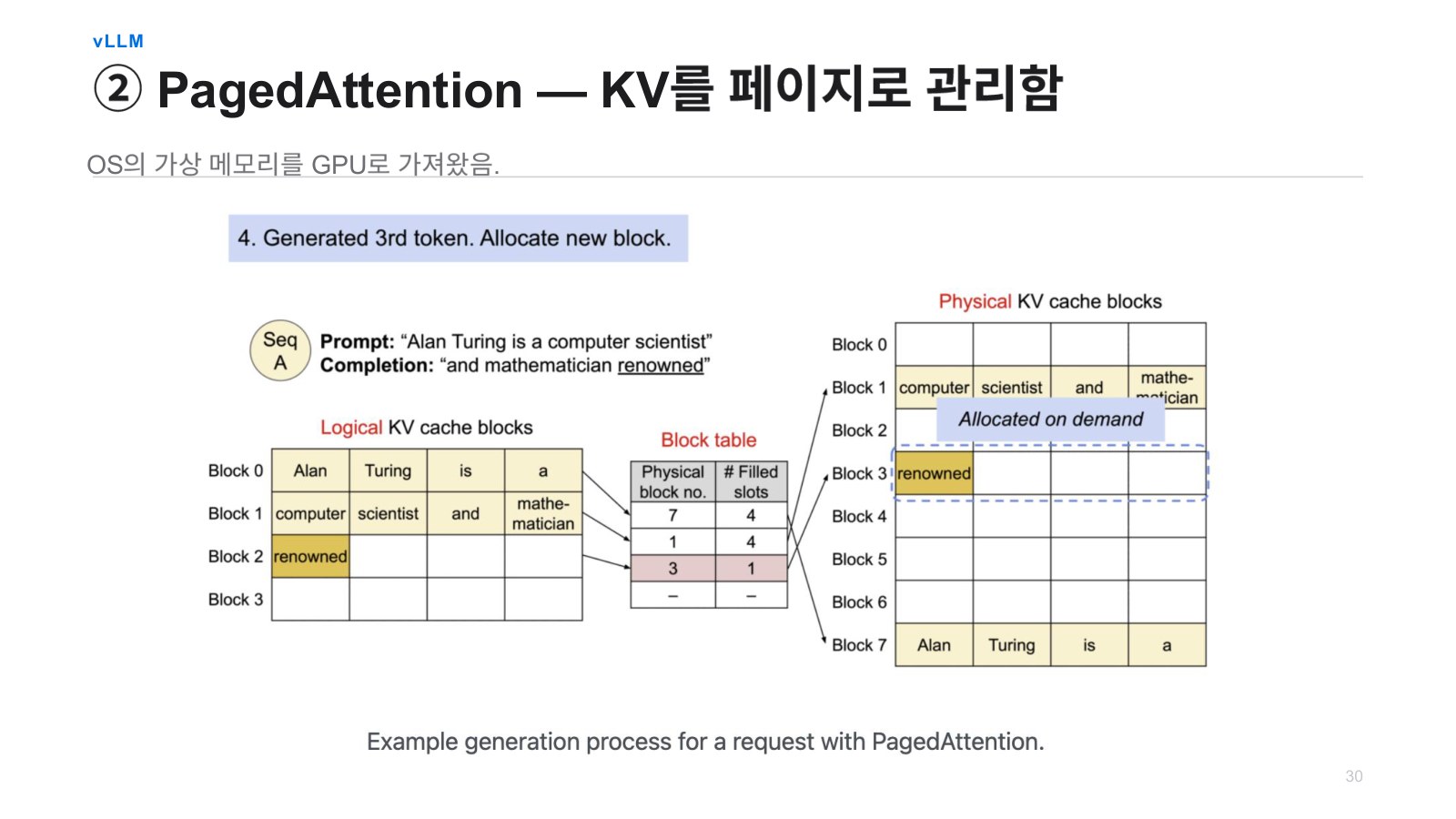
Jinwon Lee Next, there is something called PagedAttention, and what this is, is that we said earlier that we cache KV. Then we need to store KV in memory, but with ChatGPT, Claude, or Gemini, we do not know how many tokens or words they will use in their response. If we knew how many words they would answer with, we would know that that much KV would be produced and allocate that much memory in advance, Because we don’t know that, the amount I can generate worst case, when I generate the maximum amount, when I give the longest possible answer, is what I have to use as the basis for allocating memory space. Until that request is finished. Then, in reality, the memory, as you mentioned earlier, for people who just have short conversations like “Hello,” will end after just a few words, a few tokens, so all that remaining space would be wasted. So, the idea for reducing that waste, is also very simple: dynamically allocate memory. You bring in the concept of a page table. For example, if the first output word is the word Alan, to store the key and value for the word Alan, you allocate memory space in actual physical memory to block number 7. But since this space is a page, for example, it can store up to four words. If Alan comes first, you store the key and value here, and then if Turing comes next, there is an empty slot beside it, so you keep storing them. After storing them until a comes out, if the word computer comes out, the page is full, right? Then you allocate a new page at that point. So block number 0 here is now linked to physical block number 7. Block number 1 here is linked to actual physical block number 1, and block number 2 is linked to number 3, but this filled slot currently has one slot occupied. So it tells you the information that there are still three empty slots. So, dynamically like this, if you allocate a new page in memory as needed, you can use only exactly as much memory as you need, making memory use efficient, so you can provide services to more users. That is the concept.
But while this also seems like a good idea, it is not simple either, because in the worst case, although it is very rare, if everyone, in the worst case, produces maximum-length output, a problem arises. Because this is kind of like this: since people do not withdraw their deposits from a bank, the bank keeps a low reserve ratio, whereas normally, assuming the worst case, it should reserve all that memory space and serve only that much, but since not everyone will use that much anyway, it accepts additional users. But then, if all users produce the maximum output, memory space will run short. Then you have to evict this KV, and load it back in later, so it is not very simple from a software perspective. But in most cases, that does not happen very often, so it can be used effectively.
Chester Roh Those are the areas where deep engineering comes into play, and we might think that if we only use NVIDIA GPUs and run open-source models, anyone can do business, but depending on how well you optimize within that, the figures can really vary by several orders of magnitude. We call that area the orchestration software layer, and it includes things like vLLM and SGLang, Kubernetes, and many other things, in it, so not only hardware, but also this infrastructure software area is an industry area that we should pay very close attention to, and I definitely wanted to mention that.
Seungjoon Choi That is what it does.
Jonghyun Park I understand that PagedAttention was published as a paper, then it became open source and became vLLM, and it has probably been applied to nearly every inference serving framework by now.
Chester Roh They imitate one another, so now they have all become the same.
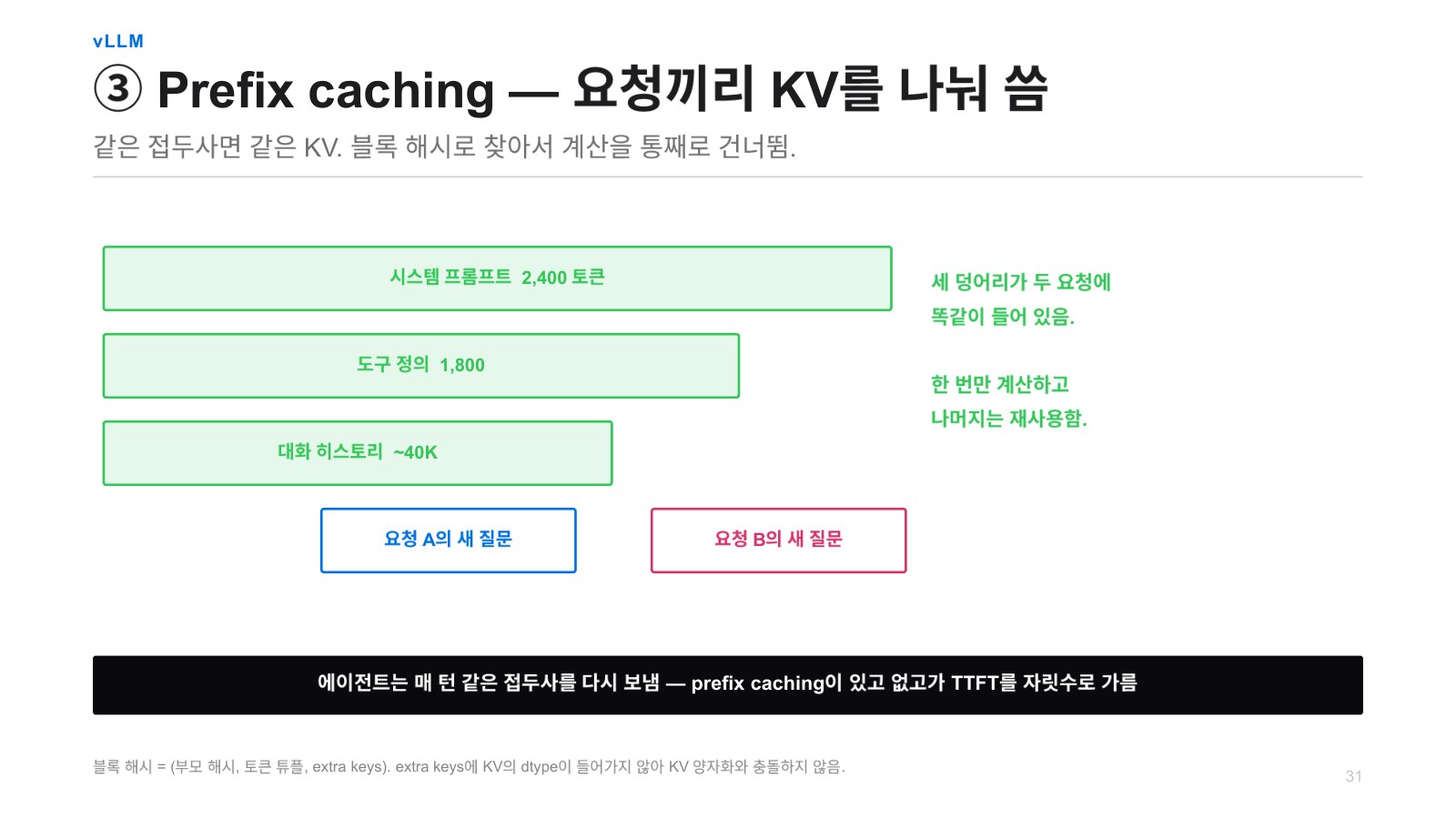
Jinwon Lee And prefix caching also is shared no matter what request comes in, so you calculate the KV in advance, store it, and simply retrieve and use it.
Chunked Prefill and Speculative Decoding 69:37
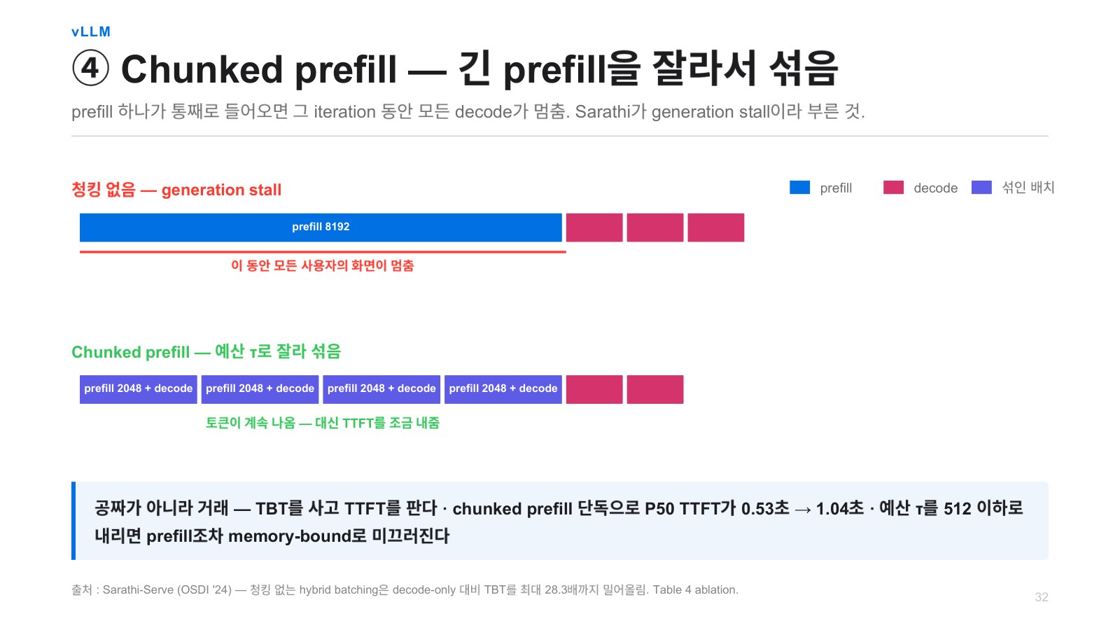
Jinwon Lee Then there is something called chunked prefill. If prefill cuts in midway, it can slow down decoding because of this. Something that could have been done quickly if this were not there, can be slowed down when, because of this, a prefill of 8,192 tokens comes in all at once. If you group these four together and put them on the bus, they are slowed down because of this. Since the ridge point earlier was only 300, to process this much, you have to run a great many iterations, and by that amount, these become slower compared with when this is not there.
So what you do about this is, you simply cut everything into the same size. This really is the bus concept: you cut it up and put this prefill in divided pieces as well. And there is a priority order when doing this chunked prefill, and in most cases, decoding is always given priority. If there is decoding, you put decoding on first. Onto the bus. Then, among the prefill requests that were cut up, the earlier prefill has gone, but the prefills that couldn’t get on the bus, and finally, the newly arrived ones— if there is still room, the newly arrived ones are accommodated as well. There is a priority order like that. That way, service quality can be satisfied best, so that is usually how it is done.
So, as shown here, it lowers TBT, and TBT is related to decoding. At first, this AI model starts answering and is answering well, but then suddenly stops in the middle— that situation happens because of this, so the idea is to reduce that and instead sacrifice a little of the time until the first token of prefill comes out. This is necessary to keep quality consistent, so this method is widely used.
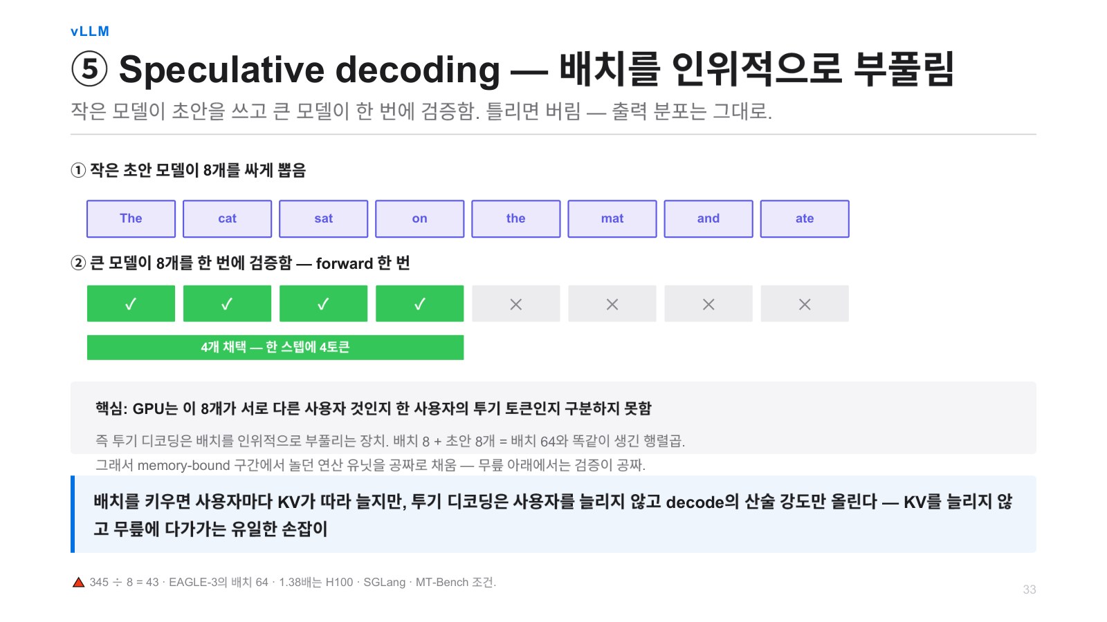
Lastly, there is speculative decoding, which Noah also talked about a lot last time. DeepSeek introduced a good method called DSpark, which greatly increases speed. The idea behind this is also very simple. In an autoregressive decode step, we generate one token at a time. The question is whether we could generate multiple tokens at once instead.
So what does that mean? Put simply, we wanted to increase arithmetic intensity in decoding by increasing the KV batch, but then the key-value pairs increase along with it, so attention did not benefit much. But without increasing that batch, a way to increase arithmetic intensity is to generate multiple tokens at once. But generating multiple tokens at once is not easy. Because they all have dependencies; if you generate the second token without looking at the first token, accuracy will naturally drop dramatically.
So this is how the concept initially started: rather than doing that, you take a small model, roughly one hundredth the size of the original model, and run it sequentially at high speed. For example, it runs quickly and produces eight tokens like this, then you take those eight tokens to the large model, the original model, and verify them all at once.
So how do you do that? You verify them as if they had simply entered the prompt prefill phase. Of course, there may have been more words, more tokens before this, but you take all of that, rather than just the one you originally used, and process them all together.
Then, just like prefill, you process them all the same way, and when generating the next token at the end, in the original prefill, from this last word, you only generated the next word, but instead, this one also generates the next word, this one looks at these two and generates the next word, this one looks at up to these three and generates the next word, and this one also generates the next word, generating the next word to see whether “cat” comes after “the.” This one confirms “the” was right, and this one confirms “the cat” was right, and then checks whether sat comes next, verifying things this way.
So everything proceeds in parallel, and if only the LM head is processed sequentially at the end, you can examine all of this at once very quickly. So as it goes along, the cat, sat on, if “the” was not correct here— no, if mat was incorrect, if it was not mat but bench, then you recognize it was correct up to bench and go back to this small model, which is called the draft model, and send it to the draft model. Then the draft model, after bench, quickly generates another eight words in sequence, the large model verifies them all at once, and if you keep repeating this, you can make serving much faster. This is speculative decoding.
One drawback is that you need to use two models, continuously running the small model once and the large model once, going back and forth like this, which makes it difficult to run, so within the same model, there have also been approaches that make it act like a draft model and then verify again. There was research like this as well.
Meta had a paper like this. Suppose we have a model with 100 layers. Do we really have to go through all 100 layers to accurately predict the next token? For some easy words, perhaps even 10 layers would be enough to predict them. So they compiled statistics for all of that. They cut the network partway through, for example, taking a 100-layer model and cutting it down to 50 layers, attaching an LM head to it and making predictions, then checking how accurate they were.
So they compiled statistics on which layer first correctly predicts the actual answer, and found that, for example, by 70 layers, it gets almost everything right. But even by 50 layers, it gets 70% right. Then you can simply go only up to 50 layers, make a quick prediction, and verify it once, and this way, within the same model, you can make predictions quickly and verify them too. You can do it like this. There are methods of this form as well.
DSpark uses a somewhat different method, for example, using a form such as a diffusion transformer, and a diffusion transformer does not generate tokens autoregressively; instead, it produces multiple tokens all at once. Then you can use that as a draft model and do the verification with the original model. This approach can also be used.
Seungjoon Choi What is EAGLE-3, besides DSpark? It comes up here too, and I see it from time to time.
Jinwon Lee EAGLE-3 is also simply a model that does speculative decoding.
Chester Roh From our listeners’ perspective, why on earth we do this is what matters, and everyone is now working on the problem of how to continually balance prefill and decode to increase the number of tokens generated per unit of electricity cost and per GPU. That’s the problem everyone is trying to solve right now, and the reason for doing speculative decoding is that prefill is much cheaper than decode. So because decode requires so much effort, a cheaper model runs decode quickly, and then its predicted answers are put into prefill, into the large model’s prefill phase, where they are verified all at once to see whether they are correct, in an attempt to gain an advantage in the process. I think that is how you can understand it.
Seungjoon Choi And even if the currently observed ridge point is around 300, even if it rises further, this system still holds, right?
Chester Roh This is how it will work forever.
Jonghyun Park And something that occurs to me as I look at this, as with PagedAttention earlier, and speculative decoding, and algorithmic methods for shifting certain operations between compute-bound and memory-bound, as well, is that they all feel like methods traditionally used in CS fields such as CPUs and operating systems have been adapted to LLMs and GPUs. The essence of optimization keeps being reused. So it seems that knowing the old things well also helps us understand future things well.
Jinwon Lee And one thing I would like to add is that if you look at something like DSpark, the DeepSeek folks are extremely good at recognizing that this verification, too, can actually become overhead. Because right now, only four in this diagram are correct, and four are incorrect, but as you go further back, the likelihood of being wrong increases. It is a waste to spend computation verifying the ones at the end. And computation is already running at full capacity, so it is wasteful for this to come in and perform useless computation. So they look at the state of the current compute resources to decide how many to verify; if compute is particularly constrained, for example, even if it generated eight, they exclude the last two and verify only six, adapting to the situation to control how many tokens they will verify. I think I was quite surprised when I saw that. I thought, “They optimize even things like this.”
Jonghyun Park And it predicts those tokens and verifies whether they are correct, but tokens, in fact, are generated probabilistically, so once you set this threshold, because even if A is generated as a token, even if “Hello” is generated, or even if “Greetings” is generated, both could be considered correct. So even if it is not the token with the highest probability, if it is a token with a fairly good probability, you could simply treat it as correct and move on. That is also something we can control. So it seems entirely possible to sacrifice quality in ways that are not noticeable while increasing the token count, and I understand that this is already being done extensively in practice.
PD Disaggregation Separating Prefill and Decode Pools 78:53
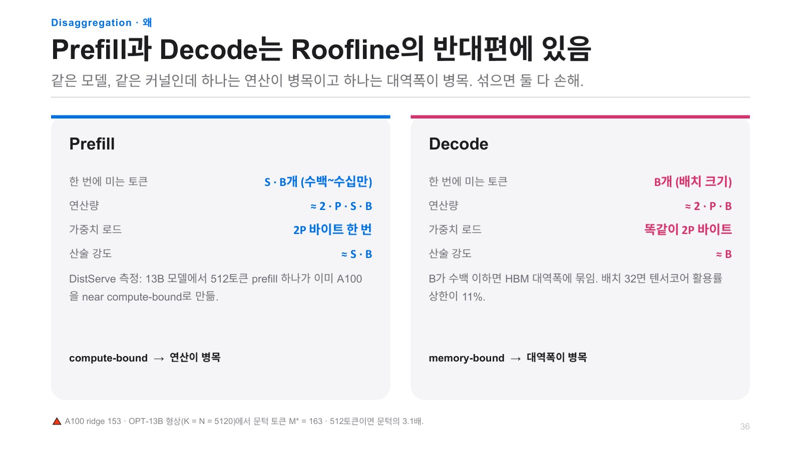
Jinwon Lee Let’s move on. I would like to talk a little about disaggregation. But we have kept saying that prefill and decode are very different, and that arithmetic intensity is affected by sequence length times batch size, while decode, excluding attention, is affected only by batch size. That is how we understand it. So we could see that they are very far apart on the roofline. So as I mentioned earlier, even if you do chunked prefill, whenever prefill comes in, decode has a different nature, so a lot of prefill affects decode, while if you prioritize only decode, prefill’s TTFT gets worse. So the simple idea was to split them up. That way, we can meet the required SLO with throughput—what we call goodput— and increase goodput.
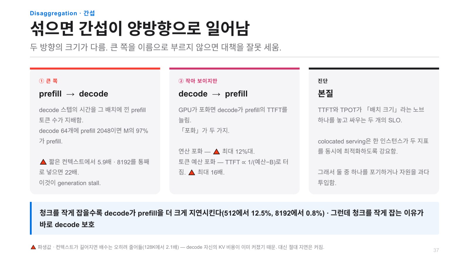
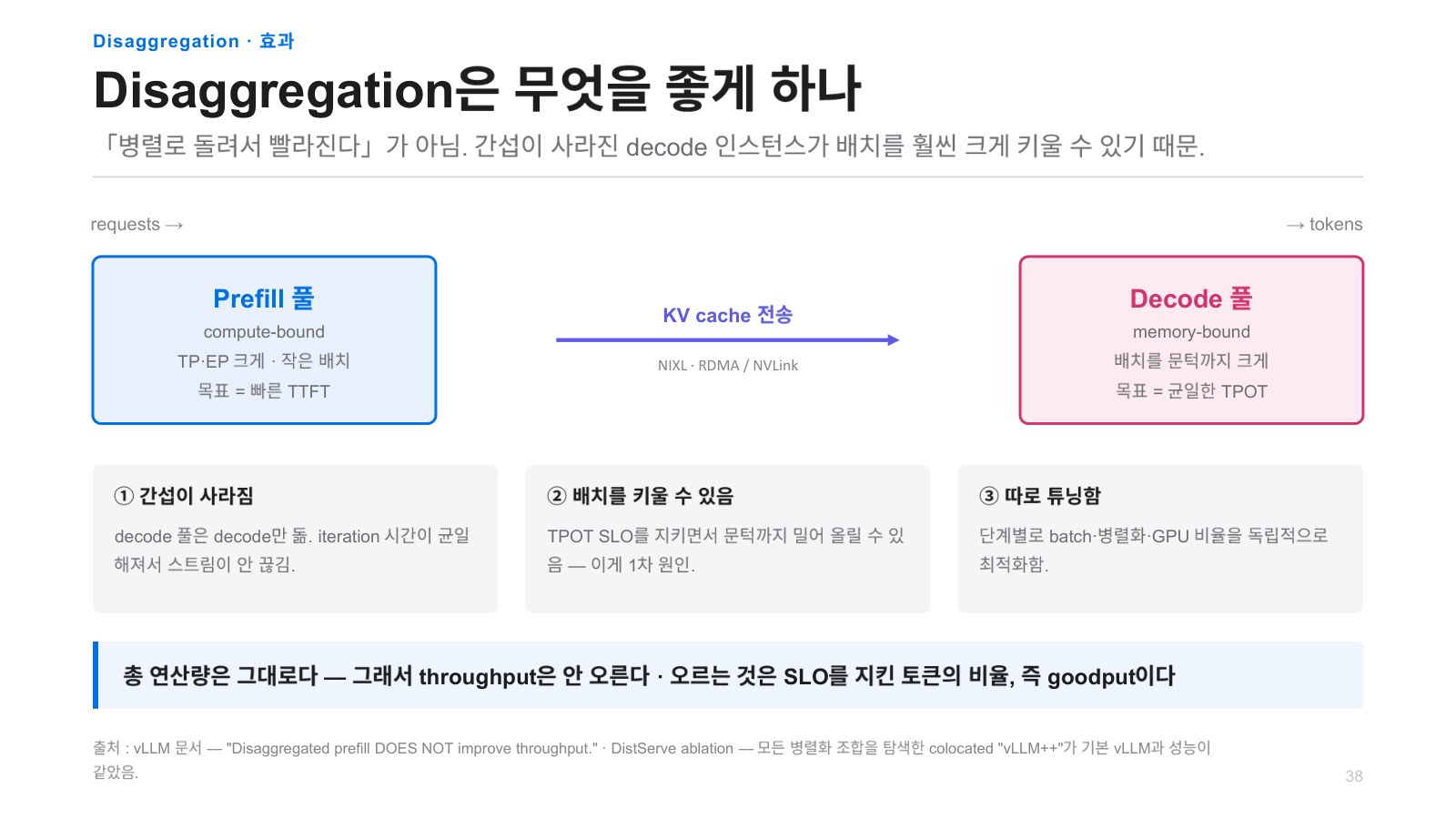
So you set up a prefill pool and a decode pool and split them up. Jensen Huang often talks about a Token Factory. I think that includes this aspect as well: it may mean generating many tokens, but more than that, it is like making cars on a conveyor belt, where one person assembles the wheels and another person installs the doors. For each individual stage, you create a pool that does only that one thing. So you separate a prefill pool that only does prefill and a decode pool that only does decode, and call this PD, prefill-decode disaggregation. Then, all the key-values created in this prefill have to be sent to the decode pool. So when you do disaggregation, the network speed between them is also extremely important. Unless this is at a certain scale, there is not much benefit. The benefit comes when there is scale.
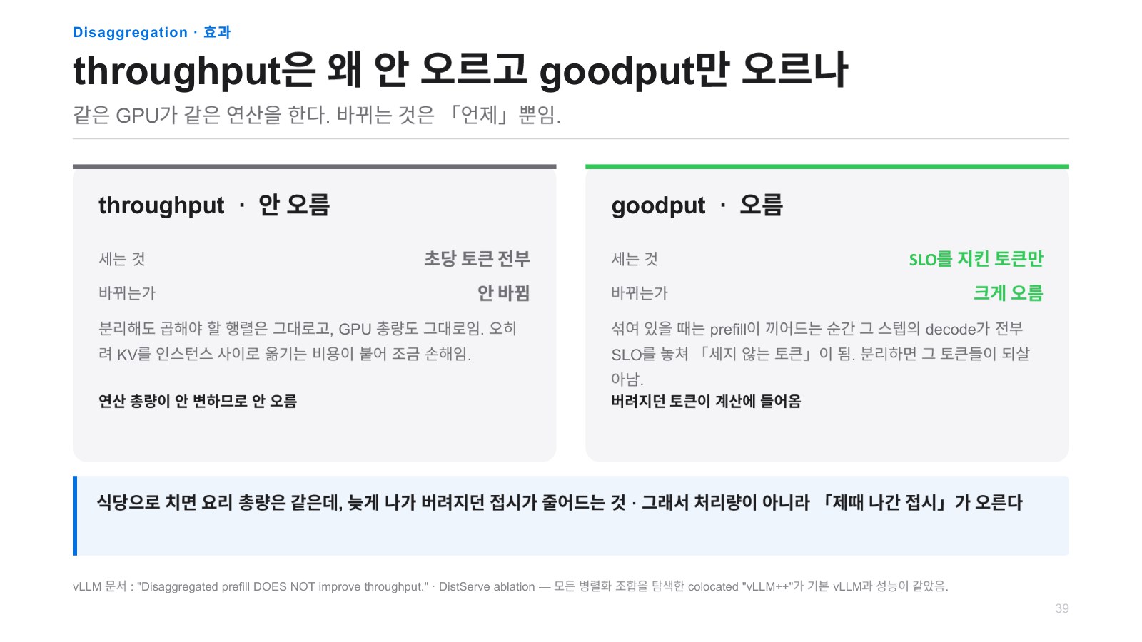
So, as I mentioned earlier, in terms of raw throughput—that is, how many tokens are generated— it does not increase. The utilization is the same. They are all running at 100%. Even if you use the same GPUs, typically, at first, in a paper from Microsoft called Splitwise, disaggregation was discussed for the first time, and as you can see here, they use the same H100 GPUs but vary the number of prefill instances. Anyway, they vary the number to match the throughput, but there is a benefit only when it reaches a certain scale. Then, if everything is running at 100%, if you have 100 GPUs and split them at some ratio, and all 100 are running, the number of tokens generated will all be the same, because the required amount of computation is fixed.
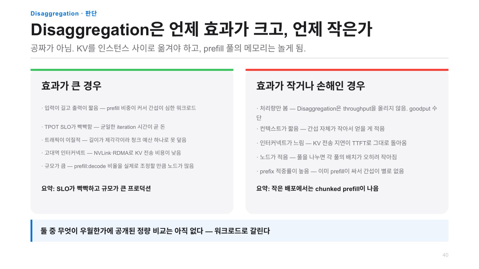
But what improves is called goodput: the throughput that lets us meet the requirement of generating at least 30 tokens per second, the throughput that satisfies that requirement increases. This increases very significantly. So these days, this is used very widely. So, looking at when the effect of disaggregation is large and when it is small, for the effect to be large, when inputs are long and outputs are short, the prefill portion is large, so decode is heavily affected, and that is when it can be used. Also, when the SLO is very strict and tight, and there is something like, “We must absolutely meet this,” it is good to use it, and ultimately, you need a high-bandwidth interconnect, so that is the summary for large-scale cases.
In cases where the effect is small—conversely, at a smaller scale— simply using the chunked prefill method can in fact be more advantageous. And it is particularly heavily affected by the interconnect. So, because NVIDIA GPUs have very high-speed networks such as NVLink, this works very well with NVIDIA GPUs, but if there is an AI semiconductor with a much slower interface than that, the benefit of this disaggregation may be less than you would expect— that is what I can say. That concludes everything I wanted to say about inference engineering. There is more, but I introduced the things I consider important.
Chester Roh Today, you covered nearly all the essential parts of inference engineering. In that roofline discussion, you explained what optimum point should be created between compute and memory, and then between interactivity and throughput, you discussed the trade-off, and then you went through all kinds of techniques, all the techniques included in this, and everything you mentioned is already in current production, right?
That’s right. And it continues to evolve today, and you need to understand all of this to make chips as well.
New Inference Workloads Created by Agentic AI 83:33
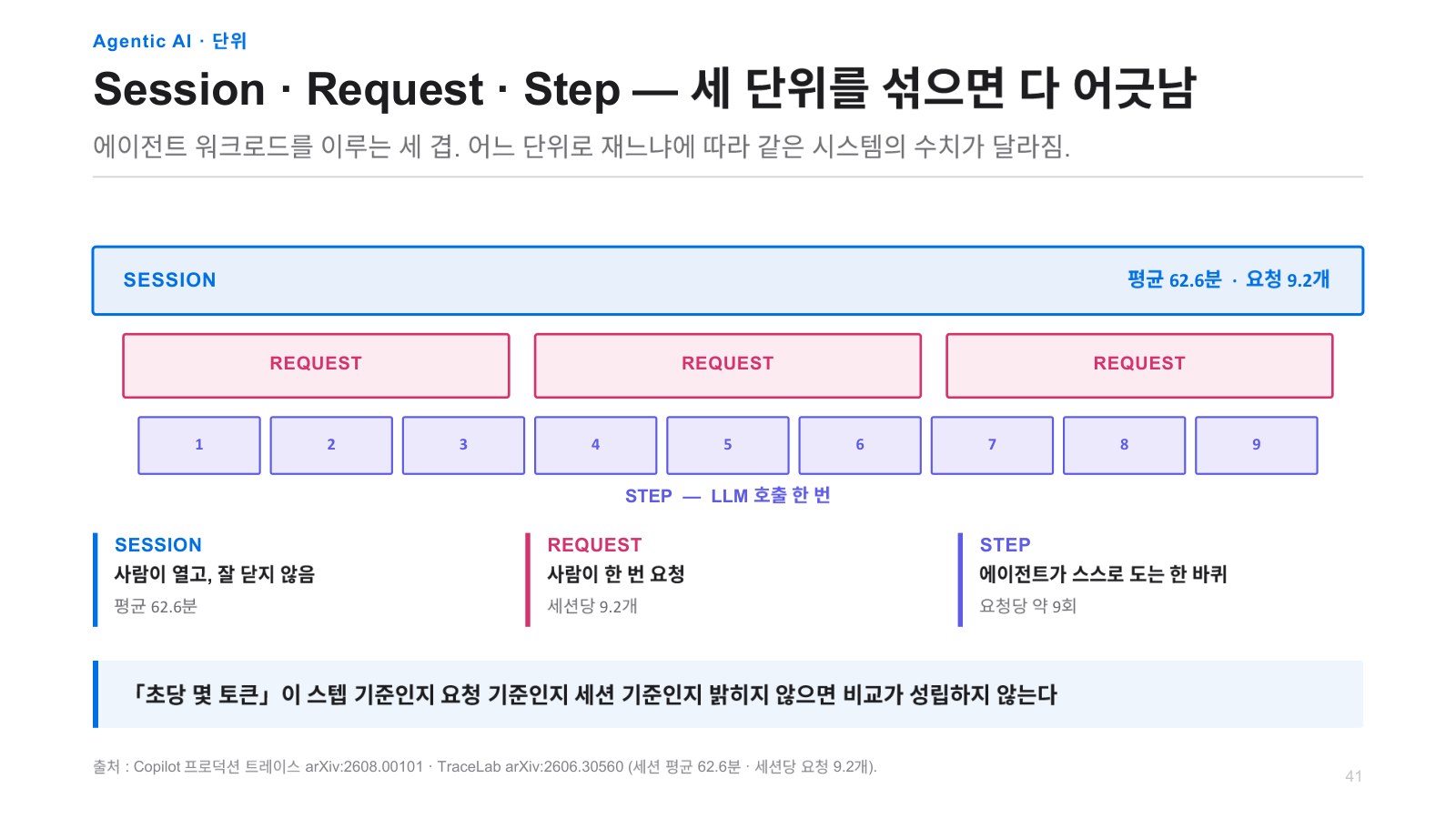
Jinwon Lee So next, this part is about when we use LLMs simply as chatbots or for reasoning to that extent, but with agentic AI— I also use AI agents very extensively— things change a little when agentic AI arrives, so conceptually, things may change like this. So these days, papers analyzing the workloads of AI agents are suddenly coming out in large numbers. Recently, as you can see below, there is also a paper published in August that analyzed all of Copilot’s traces from the single month of June 2026, and there is also something called TraceLab, and so on. I referred to these papers.
To organize the terminology, if we look at session, request, and step, a session is when we start an AI agent until the agent completely finishes; you can think of that as a session. Within that, a person gives a prompt for a request, and the AI agent runs a loop. It runs a loop, calling the LLM and calling tools, until it produces a result—that is one request. Then the person looks at it again and gives feedback and assigns another task. That next task is another request. So the beginning of a request always starts with a human prompt, and within a request, the LLM runs and tools run as well, and each time an LLM or tool is called, you can think of that as a step.
So, looking at the statistics, a session averages 62.6 minutes, and there are about 9.2 requests per session. Within each request, there are about nine steps, so, roughly speaking, if you calculate it for one session, you can think of it as containing about 100 steps. Naturally, of the actual LLM calls, most of them—about 90%— these two red 90% figures show that AI made the calls. In other words, AI uses AI more than humans do. When a person enters a prompt, the LLM is called by a person only once at that point, but while the agent is running its loop, the agent keeps calling the LLM.
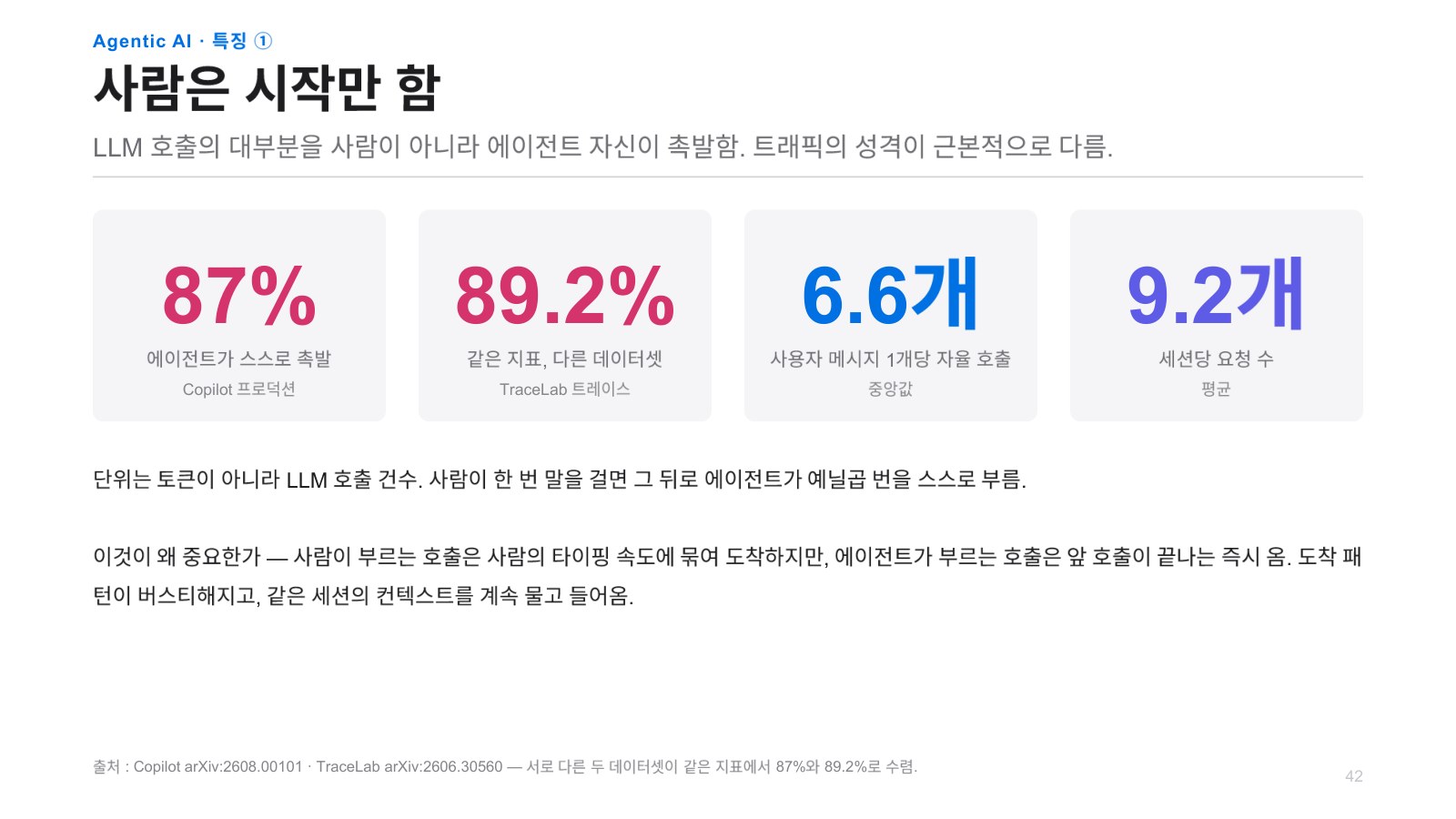

And this goes through an enormous number of interactions, and there is also a reasoning process in between. As we moved from using it as a chatbot to reasoning, we started generating a huge number of thinking tokens. So the length got longer, and accordingly, as we discussed earlier, the KV cache space also grew, but now, an LLM call that performs reasoning gets included in each step of this agent. Then it will multiply several times over again. When you look at this LLM running, reading the KV cache that had accumulated beforehand accounts for almost all of it, and 119,000 tokens come from the prefix—that is, from reading the KV cache calculated earlier, while 875 are newly added, and the resulting output tokens are 214. That’s about one hundredth of the amount. So to that extent, rereading has become extremely important.
Another important thing is that all of these workloads are heavy-tailed. We call it long-tail, but it is a heavy tail where the tail has a huge impact. So if you ignore the worst case, agent services will fail. So you always have to consider the worst case, and what makes this clear is the skew between the median and the average, which can differ by as much as 15 times. There is also analysis of things like weekday versus weekend usage, and naturally, usage is much higher on weekdays. There are more sessions, whereas on weekends there are fewer sessions, but there are far more iterations per session. So naturally, people are likely running more complex jobs over the weekend before going home or doing something like that, and if you analyze a single session,
Human-Created Latency and the KV Cache Golden Window 87:22
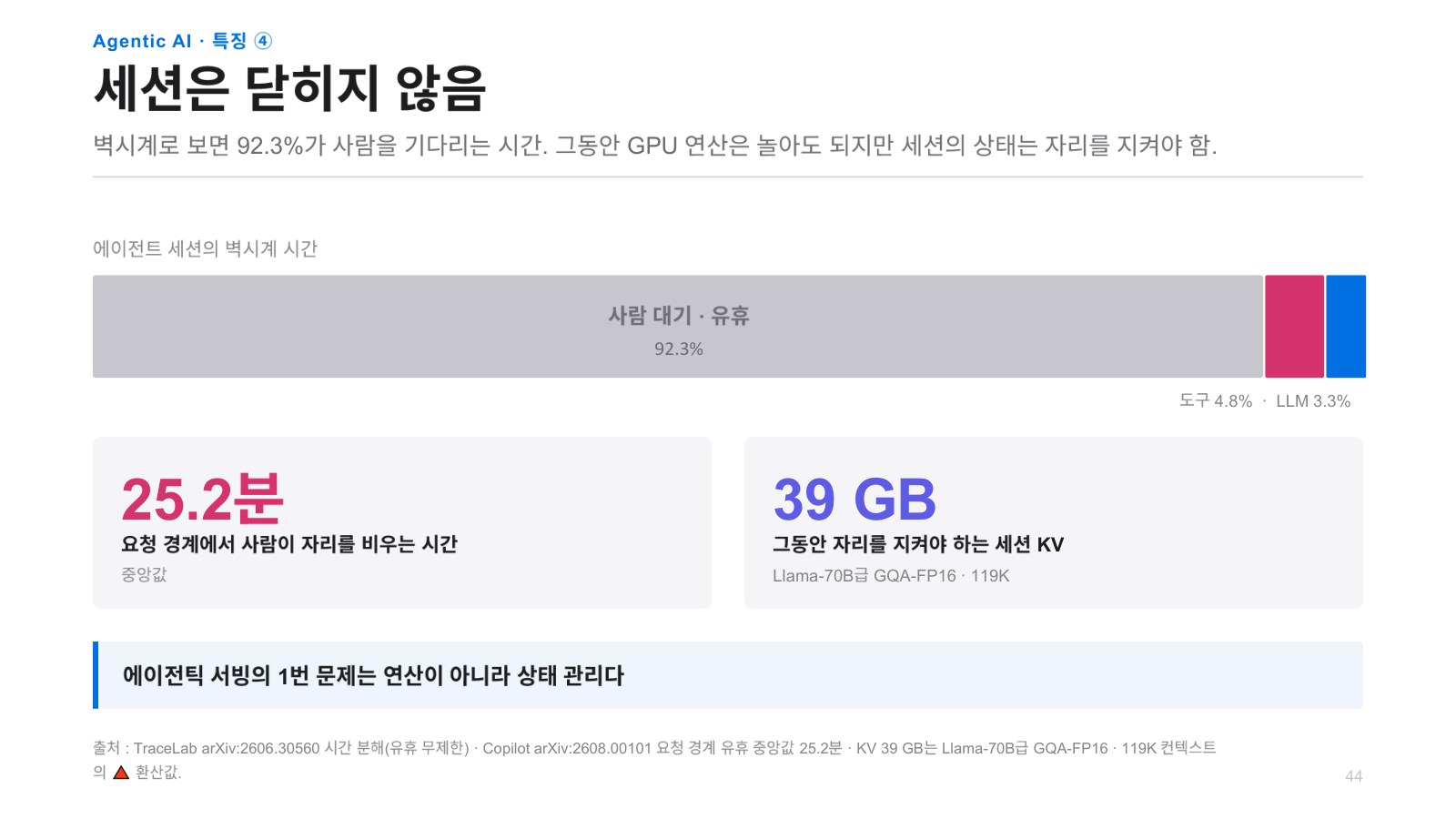
Jinwon Lee between one request and the next, a person has to decide, understand the result produced by the AI, and then send the next request, so there is time. Usually, in my case too, I assign work to an agent, use another agent or do something else, and when I come back, I check it thinking, “Oh, it’s all done,” so people are not watching the AI continuously work. Most of the time, they come back after doing something else, so a lot of that time is wasted. So people occupy about 92% of the entire session, while tool calls take 4.8% and LLMs take 3.3%, so if you view it as almost one-to-one, these actually use 8%, while people use 92% of the time. That means people are the bottleneck.
But this does not merely mean that people are the bottleneck. Then, in a situation where you do not know when people will return, do you have to keep the KV cache produced earlier by tools or LLMs in expensive memory called HBM, continuously? That is the problem. So within a session, the median time a person waits between requests is 25 minutes. Holding this KV cache for 25 minutes is extremely wasteful. And during that time, the median KV cache capacity that remains in place and occupies that space is about 40 GB.
So after around 25 minutes in most cases, it is all evicted now. It is sent to somewhere like storage, and five to ten minutes is the golden time. Based on the current analysis, it is kept until about then, but beyond that, this is also predicted. This uses a very lightweight machine learning model to predict whether this person will return within 10 minutes or not, and if they do not seem likely to return, it also uses a method of evicting it quickly, and they say its accuracy is higher than expected.
Seungjoon Choi Is it trained for each user?
Jinwon Lee Whether it is done per user, or simply based on the content.
Jonghyun Park If you imagine it simply, before going to bed, people run something for a very long time and go to sleep, so the time until they wake up in the morning is extremely long. So what time it was run would likely have an effect, and what task was assigned would likely have an effect as well, and simply classifying those things would probably improve the accuracy tremendously.
Jinwon Lee According to that paper, predicting how many minutes later someone will return is somewhat difficult, but whether they will return soon or not return soon is still predicted fairly well.
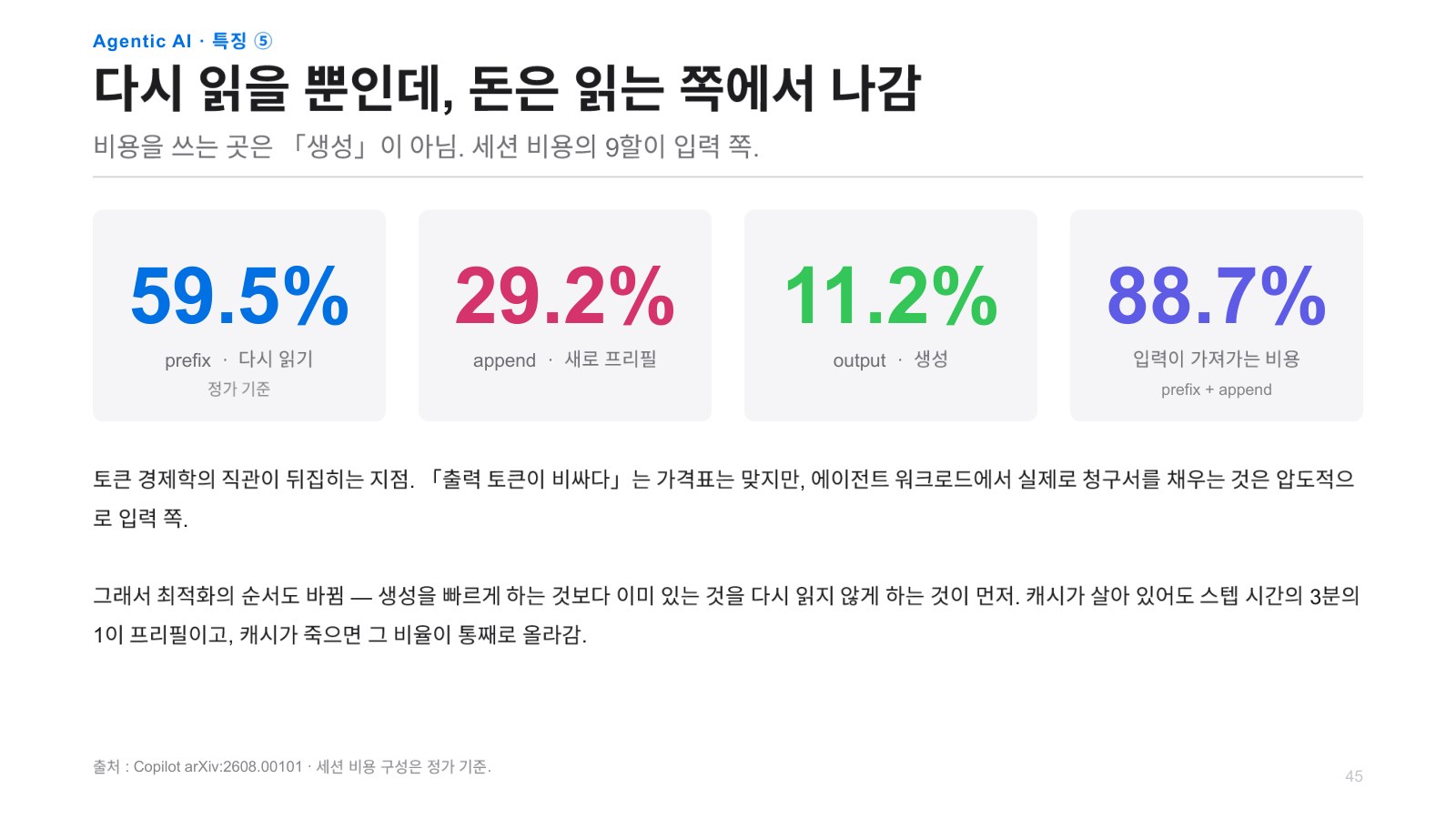
Chester Roh Agent workloads are not compute-bound; they are overwhelmingly memory-bound. Calling them bound almost feels beside the point—they are simply memory work. It is a game of holding things.

Jinwon Lee So in the end, rereading it also costs a lot. If you calculate this as well, based on renting services in the cloud, 60% becomes the cost used to read the prefix. Then, when this is evicted, you could delete it entirely and then, when the user returns, recalculate the KV cache. Or CPU DRAM, or send it to storage, and then read it back in. When comparing those two, if you ask which is better, in almost all cases, it is better to put it somewhere far away and read it back in. Recomputing it takes a long time and costs a lot, whereas reading it back takes some time but is much shorter than that, so it is more advantageous, and that is the direction we are moving in.
Reloading KV Cache Instead of Recomputing and Hierarchical Memory 90:10
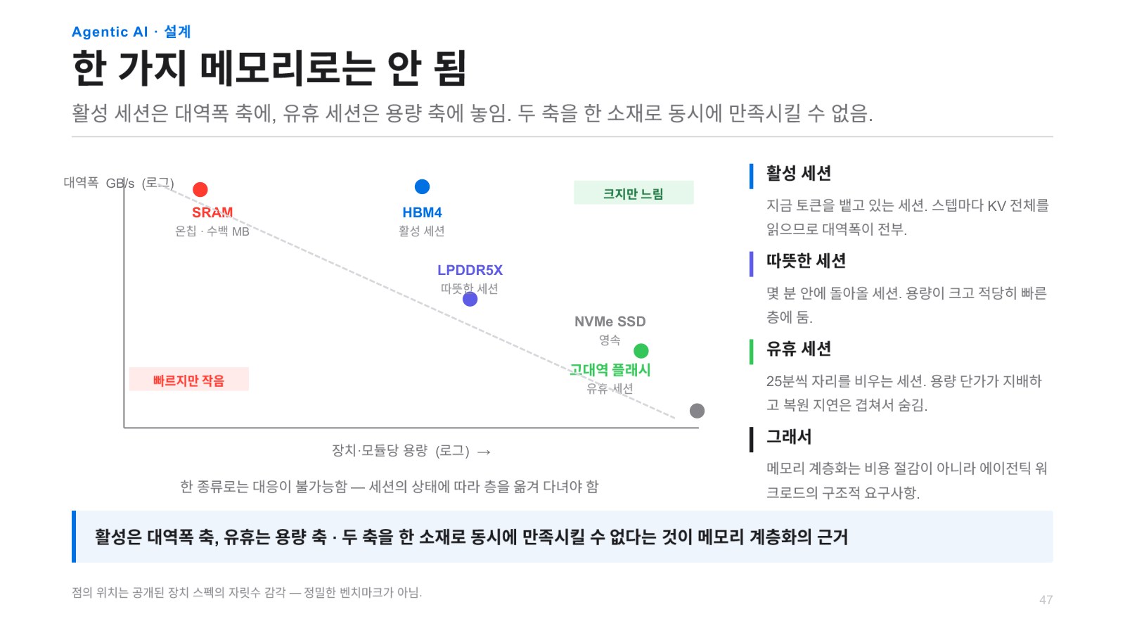
Jinwon Lee And while reading it back in, if you can perform some computation, that latency can be completely hidden, which is even better. That’s the idea. Now we also need to use memory hierarchically, SRAM, HBM, DDR, SSDs or things like high-bandwidth flash are being discussed a lot these days, and it is important to divide up all of these roles well for the intermediate results of the KV cache, scheduling how and when to send them where, and when to bring them back is newly emerging as something extremely important in agentic AI. Then more open-source tools that do this well, software such as vLLM or SGLang mentioned earlier, will emerge going forward. So the bottleneck moves from compute to memory, then to power, continually going back and forth like this, and the answer changes each time, and whenever there is a bottleneck in one area, people try to solve it by whatever means they can. That’s what I wanted to share today.
Chester Roh People are making them do an enormous amount of work, but most of that work, from the cloud’s perspective, is a game of remembering things, and requires very little computation, as you said. Then, from that standpoint, demand for memory companies will continue to grow for quite some time, and because they will also optimize a great deal within that, the margins of companies providing this kind of inference work will likely remain quite high to a significant extent.
Anthropic and OpenAI will likely continue to become more profitable.
Seungjoon Choi For example, while running a context agent workflow, the context gets compressed. Then you would keep only the final compressed KV. There is no reason to keep what came before.
Jinwon Lee You end up keeping only the compressed KV. Some things can also be lost in the course of compression. So at that point, there are cases where you need to do the computation again.
Chester Roh But compacting is unavoidable because of limits set by the model, so the important thing is that each cloud provider offers a different max context length right now. Some offer Opus 1M, 1M, one million tokens, as their context length, while others offer only 270,000 tokens, so that means they are using entirely different farms, and the amounts they charge accordingly must be set completely differently.
Jonghyun Park I am curious about how HyperAccel views its outlook or future. Because HyperAccel is also building new chips needed for all infrastructure: compute, memory, and power, and is building the chips as well as the computing platform itself. But of course, besides HyperAccel, an enormous number of teams are trying to solve all of that. Then the inference hardware market itself will continue to grow, and NVIDIA GPUs are currently used the most even in the inference market, but ultimately, including Groq, whether it is Groq, Cerebras, TPUs, or various other chips, they will all enter the market and replace a large share of it. What was that news I heard recently? GLM-5.3 Flash was also run for inference entirely on Chinese chips, or so I heard. I think that is how it was announced. I am curious how the landscape of that market will change going forward.
The Future of Heterogeneous Computing Combining GPUs and LPUs 94:21
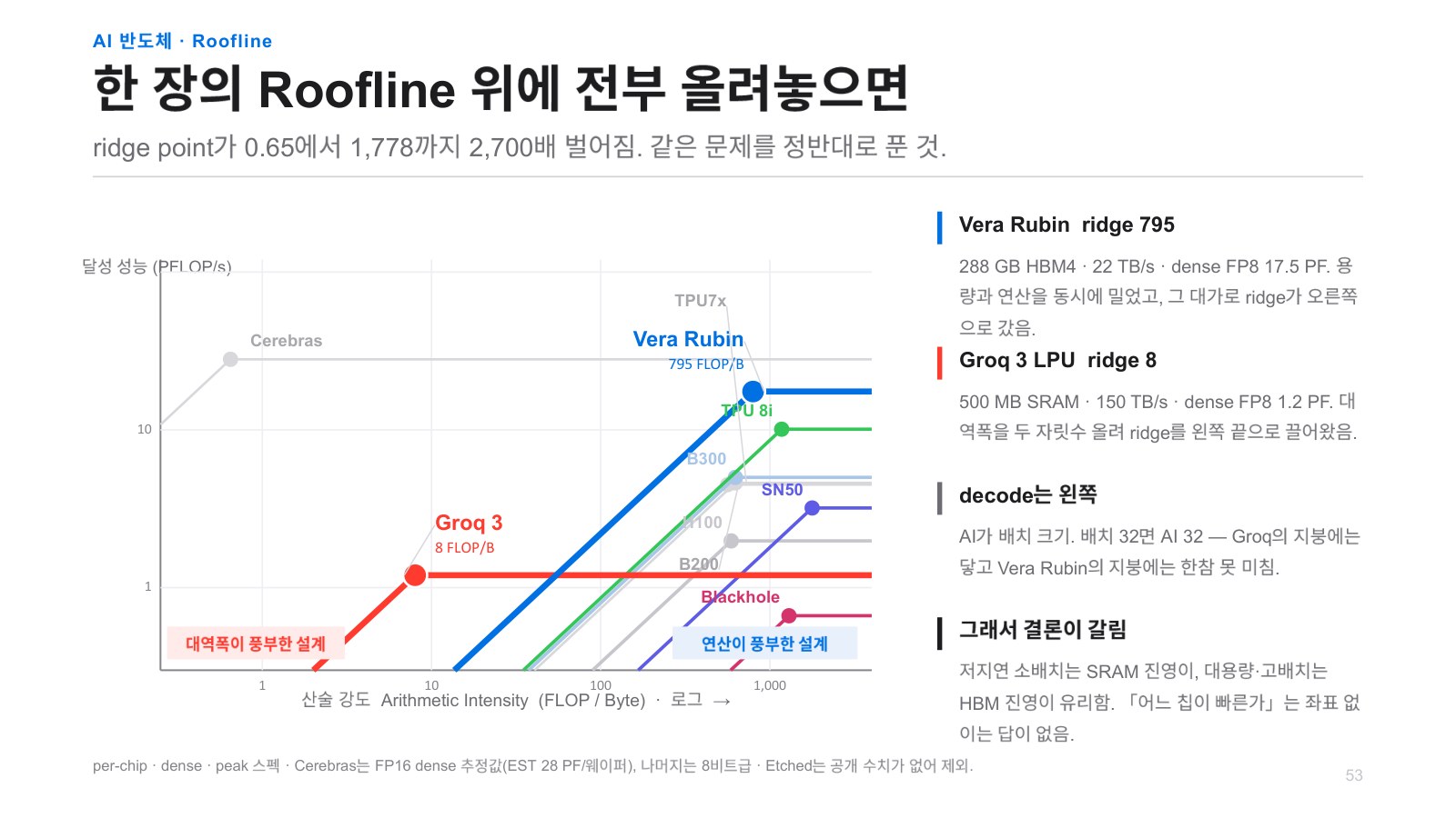
Jinwon Lee That’s a very good question, and the reason NVIDIA acquired Groq is that I tried drawing the roofline graph mentioned earlier as a graph for hardware, including a wide variety of AI semiconductors and GPUs. The Vera Rubin that I highlighted here looks like this, while Groq looks like this. As we saw earlier, lower down, you can tell that this one has much higher bandwidth because it is positioned higher up. So earlier, I mentioned prefill-decode disaggregation, and in the Vera Rubin family, they call that LPX. The role of LPX is that, even with disaggregation, the prefill is all done on Rubin GPUs, and decoding is also done on Rubin GPUs through attention, with only the FFN handled by Groq’s LPX. But its arithmetic intensity ridge point is shown here as 8. That is a single-digit number. So compared with this blue one, this red graph is higher up, in regions where arithmetic intensity is relatively not that high, which is where Groq’s LPU has an advantage. So InferenceX mentioned earlier is also positioned in that region on the right.
But Groq uses only SRAM, and it is about 500MB, The chip that joined this Rubin family this time, then 500MB is a very small size, right? So all those KVs we talked about earlier can’t fit in there. Of course, to fit them, you’d have to use an enormous number of chips. As a result, FFN doesn’t have KVs, right? So that’s one reason it’s suitable for that, and another is that even with FFN, if you increase the batch as mentioned earlier, by as much as you increase the batch, it’s an area where you can raise arithmetic intensity, so you might think it isn’t suitable there, but with the arrival of MoE, the batch is divided among the experts. So from the perspective of a single expert, the batch size becomes relatively smaller. So arithmetic intensity there still remains low. So it becomes a solution that is very well suited for that. There is no need to pass KVs to one another, and between the GPU and LPU, there is almost no need to transfer that data, because only these tokens need to go back and forth, so it’s a very smart solution.
So if there are clearly advantageous characteristics, they can be incorporated into this inference pipeline, serving pipeline, for example, depending on the characteristics of agentic AI going forward, we might be able to retrieve data from external memory extremely quickly, or there might be an enormously large external memory attached close to this chip, if there are characteristics like that, we could send KVs there and use it as storage space while performing some computations as well. If there are characteristics like that, when they fit well into this pipeline, things will operate in a highly heterogeneous way. That kind of world will come. Homogeneous computing is nearly over, whatever it may be, work will be done to find what each does well and plug it in. So for us at HyperAccel as well, our first product focused on price and power because we thought they were major bottlenecks, if that was our focus, we are now preparing our next product. It will fit well with the characteristics of agentic AI.
AI-Driven Changes to Semiconductor Design and Verification 97:54
Seungjoon Choi With this Jalapeño as well, there are similar nuances in other cases, and I’m wondering whether RL tasks in chip design are moving into verifiable areas.
Jinwon Lee That’s also very interesting, and it’s one of the areas I’m most interested in. Because I often say, almost habitually, that in about three years I don’t think I’ll be able to do this work anymore. I say that a lot, because I believe AI will do it much better than I can. So what is somewhat fortunate is that it has been built on FPGAs, and I think papers have been published as well, and it works extremely well, more than expected. There are also quite a few verifiable areas. It won’t be easy for the entire thing to come together all at once, but already, parts of design, and especially verification— whether what I designed works properly— are entirely in the software domain. But design involves coding in languages such as RTL and Verilog, while taking hardware into account, and because you have to code in a hardware-aware way, there are things to consider, and the criteria for evaluating whether the result is good, whether it was made well or poorly, can vary greatly depending on the case, so there are difficult aspects, but in any case, there are metrics, so I think it is verifiable. I think it’s a matter of time, because ultimately, it’s not a matter of whether you only need to design well or only need to verify well. Based on that, you also need to do things well physically, at the transistor level, including layout, P&R, place and route, and there are many very complex problems.
So all those things have to come together for a good semiconductor to emerge, and for a semiconductor that operates properly to emerge, so I think it will take a little time, but I also think it won’t be long. So if you look at OpenAI as well, with things like software, especially while talking a lot about CUDA, they said that CUDA-related things were all quickly built using Codex. For example, something like MLA didn’t have a kernel, but in order to run DeepSeek, Codex quickly made it all, they said things like that, and seeing that, it seems like it won’t be long.
The Warring States Era of Specialized AI Chips 100:08
Jonghyun Park Listening to this, what occurs to me is that producing hardware itself, once you make it, is extremely expensive, so before tape-out, simulation software for verification and things like that are extremely well developed, right? So the tools that allow AI to run verification are well prepared in software, so it seems like AI could create those things well, and as Jinwon explained, hardware has its own trade-offs, so hardware for specialized purposes, like Groq, will continue to emerge, and even within the single task of LLMs, tasks can be separated and divided up according to the trade-offs. This goes to Groq, this to GPUs, this to Cerebras, this to whatever hardware, because we can divide things up this way, hardware will emerge faster, and more diverse hardware can emerge faster, and work can be split up, Shall we call it a Warring States period? Instead of one GPU doing all the work, it is like when there were only CPUs, and GPUs came out for gaming, I think it is similar to that. Specialized hardware may start coming out one after another, and as I listened to the questions and answers, I really enjoyed it as well.
Seungjoon Choi Yes, it was interesting. There were interesting things even at the level I already knew, and things I newly learned
Chester Roh as well. And these elements you taught us are constantly moving toward the frontier even today. It is not just the models that are moving toward the frontier; this infrastructure is also constantly moving toward the frontier, toward the frontier, I suppose.
Seungjoon Choi Including HyperAccel, a Korean company, it is encouraging and good news that companies in this area are continuing to push forward.
Closing Remarks and the Acceleration of AI Infrastructure Industrialization 101:42
Chester Roh These kinds of developments, whether new chips come out in the future, or whenever Jensen appears, he talks about AI factories and keeps changing their configuration. And NVIDIA’s advantage seems, as Jinwon just explained, to be under attack from countless companies in every individual area, being chipped away at, or so it seems. So it will be really interesting to see how things change over the next year. If we think back to just one year ago, we were not talking about inference like this; we were simply saying, a new model has come out, that was the kind of conversation we were having. How was it trained? How was this made? It was only a year and a half ago that we were talking about reasoning models. But now, leaving all that aside, this has become fully industrialized. How can we build a profitable cloud and make a business out of it? We have reached that stage, which feels like a world apart, and the pace of this change will only accelerate on a monthly basis, so I think we need to stay alert and keep up.
Seungjoon Choi There were various stories this week, including Cursor and OpenAI fighting, and NVIDIA and OpenAI fighting, among other news. It is an intense competitive situation.
Chester Roh But something I have been receiving requests for quite often lately is this: not for research or model engineering, but simply for investment purposes, or because people want to understand these changes better, things we talk about, such as Transformers, or what CTO Jinwon taught us today, such as inference token economics, they want to learn and understand these things more deeply. So, for those people, I have no way of knowing how many there are, and I cannot create such an event just for a few people. So among those who have listened this far today, if there are people who think, “I would like to study these things more deeply,” I would appreciate it if you could express your interest in the comments. Thank you again, deeply.
Jinwon Lee Thank you for listening.
Jonghyun Park I really enjoyed it.
Chester Roh Then, for today, we will wrap things up here. Thank you.
Jinwon Lee Yes, thank you.