EP 96
LLM Inference Infrastructure and Token Economics
Dwarkesh’s new episode I studied over the holiday break 0:00
Chester Roh Today, as we’re recording, is May 4th, 2026, a Monday morning. Over this holiday period, we studied Dwarkesh’s new episode. Dwarkesh changed the format. Suddenly, Dwarkesh brought in a blackboard and started teaching while writing on it, using that kind of new format. And the content was very good. At this point, we
Seungjoon Choi It was April 30th, right? That’s right. We studied this for about three days,
Chester Roh and until now, we had always talked about what training is like, and then what model size is like, that kind of thing, but in fact, with Claude Code and Codex alike, isn’t inference becoming much more important? Right. So when we run code, we have to put in a really long context,
and that long context keeps changing constantly, and workloads like that are increasing, and in between, reasoning tokens take up a huge amount too.
Even for me, I set GPT-5.5 to x-high and put code into it while carrying out tasks, and that workload is substantial.
So the modern inference infrastructure that makes those things possible. While talking a lot about models, we talked a lot about training, but now, because a time has come when inference has become far more important than training, we need to learn in depth about how that inference happens, and this Dwarkesh episode talks about exactly that.
Today’s material is quite difficult, but it will be interesting, so we will try to unpack that content in this episode.
Seungjoon Choi Let’s get right into it. Last week, we talked about DeepSeek,
Cutting context costs shown with a DeepSeek graph 1:38
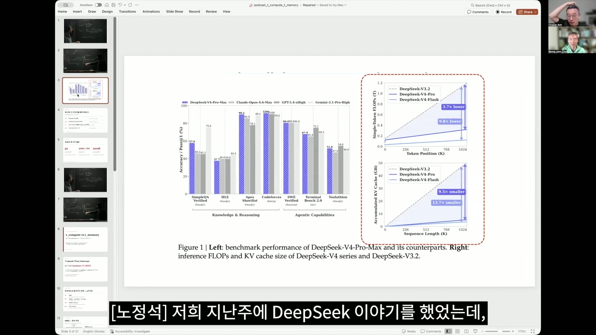
Chester Roh and actually, what DeepSeek put forward in the very first chapter of the paper was this, wasn’t it? The graph on the right is what I said was really the core of this paper, and the one above is about computation, while the one below is about memory. To summarize this simply, the token position is k,
so it represents from 0 to 1 million, and these days the frontier labs all offer a context length of 1 million tokens, but in reality, 1 million is very expensive to serve. So I understand that, realistically, tiers are mostly divided around something like 200,000, and this time I also learned why those tiers are divided that way. But DeepSeek
made things very efficient in computation and memory usage even as the context grows. It reduced computation to one-third and memory to one-tenth, and just what that means in this agent world, this agentic what do they call it, era? In this present age that is becoming an agent world, how significant that is, once you follow today’s episode, you will be able to understand.
Overview of serving infrastructure centered on NVIDIA GPUs and HBM 2:53
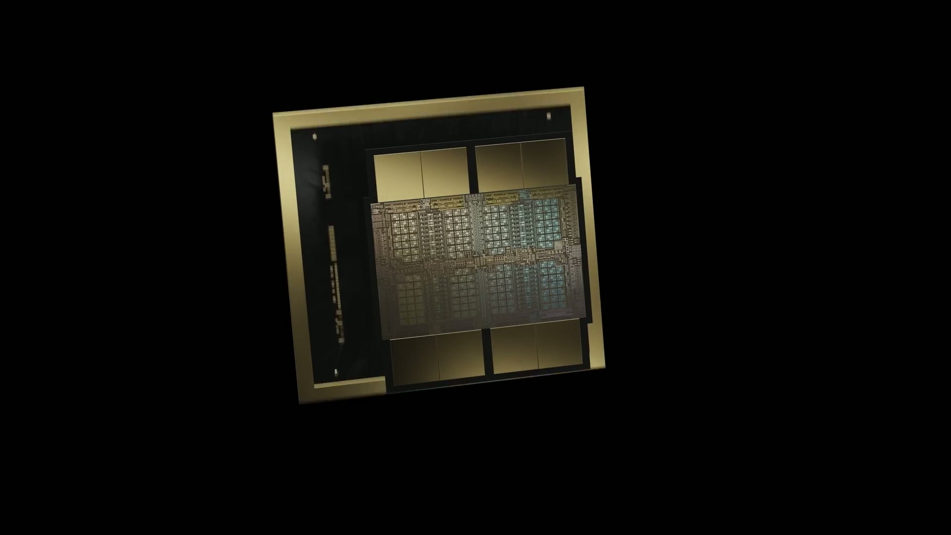
Chester Roh When we talk about models, if we talk about NVIDIA, most people do not understand it. Right. But we say there is something called a GPU, and that you need GPUs for models to run, and Jensen Huang always comes out at these events and shows all the hardware,
Seungjoon Choi Carrying it around and showing it off. Yes. There is the GPU chip, and then when there is a chip,
Chester Roh what is always discussed next to it is how much the compute units have increased, and how much faster the speed has become, and attached right next to that is HBM, which South Korea has recently been benefiting from a lot, and those are bundled together, then bundled with CPUs to become a rack, and then GPU-to-GPU communication, then rack-to-rack communication, these kinds of infrastructure are all explained one by one, but we do not exactly understand all of that, do we? Today, about those things,
we will talk about them. In fact, if we first lay out the conclusion of what we will talk about today,
Blackwell NVL72 and rack-scale memory expansion 3:52
Chester Roh communication between GPUs in this Blackwell NVL72 used to be possible only up to 8 GPUs, but now it is 72, and the capacity of each individual GPU even with the H100 or H200 that Elon Musk installed in Colossus, was only about 80GB or 100GB of memory per GPU.
But the GB200 or GB300 systems coming out now, which have been shipping since last year and into this year, have 192GB of memory, even 288GB models, and so on. And those things
are all connected as one with 72 GPUs in a single rack,
Seungjoon Choi Then how much is that? Is it around 20TB? It is around 20TB. In fact, all of those things have implications,
Chester Roh and the latest models now are using this hardware structure extremely well, and it is so related that it would be fair to say the model architecture is also being shaped by it,
Seungjoon Choi It explains why the models we meet these days changed so sharply around 4.5 or 4.6. That is what this explains. That’s right. If you look at the release timing.
And GPT-3.5 came out in October 2022, and then GPT-4.5 came out close to a year and a half to two years later, and in between, GPT-4.0 was in play for quite a while, That was March 2023, right?
Chester Roh Right. We thought of it as a model of about 1.8T. And Claude Opus 4.5 or 4.6 and things like that, according to what Swyx said, just as a rumor going around, though no one confirms it, were said to be models with a maximum of 1T to 2T. But the models suddenly coming out now are 5T models, 10T models, these model sizes have suddenly become much larger.
Seungjoon Choi Right. Mythos is 10T, and then around 5T is probably being served right now, according to many guesses. Why are these things suddenly happening now?
Chester Roh There is a reason this is suddenly repeating. So Dwarkesh and Reiner Pope, a founder who came from Google hardware, appear,
Reiner Pope’s talk and today’s roadmap 6:09
Seungjoon Choi Reiner Pope worked on TPUs. and explain it while writing on this blackboard.
Chester Roh So today, following a few parts of what is written on that blackboard, and ultimately, how modern LLM serving architecture actually works, what game they are playing, and so on, we are going to follow that long story as well. So the content of today’s episode
may feel quite difficult. But for those of you who use Claude Code or things like that and simply just want to use them, the content of this episode may not be very interesting. However, the timing of NVIDIA GPU shipments, and then the model architectures
that are shipped, and how these show the future, are leading indicators. That’s right. This is not just about NVIDIA,
Seungjoon Choi because competitors have no choice but to do similar things too, so I have a sense that these will probably become indicators
for reading the current state of the era. Today, let’s talk about that.
What token price sheets and cache pricing really mean 7:22
Chester Roh So when we talk about why we use Claude Code, and when we talk to you about cache optimization, we use these terms as if they are nothing special.
Input tokens and output tokens have different prices, and even this price difference is small in some places and large in others.
DeepSeek, Gemini, Anthropic, all have different pricing schemes.
That is different, and then caches are also different, with 5-minute caches and 1-hour caches, and all of their prices are different too. And then even when you look at something like Gemini, the context length is okay up to 200K, that is, 200,000, but once it goes over 200,000, they charge it at a different price tier. There are pricing tables like that. Why on earth these things exist,
and what relationship there is among the latest LLM serving architectures, hardware, and all these things, is what we will look at today. The things that unpack that appear in what this guy writes on the board, but the content of this board writing, after we first cover the basics, we will come back to it and look into T_compute and T_memory, and why these things are structured this way.
So from this formula, this graph is derived. Ultimately, the time it takes per batch size,
and then the pricing tables that arise per batch size, and by looking at these pricing tables, in fact, all of the things we just talked about earlier can be answered.
So the key keywords are being limited by T_compute and T_memory.
Seungjoon Choi What is T here? Time, right? Time. The time it takes to compute,
Chester Roh and the time it takes to recall this memory, through the combination of these two, all prices in modern LLM inference are determined. That is the kind of story we will talk about today. So AI models are the shadow of hardware.
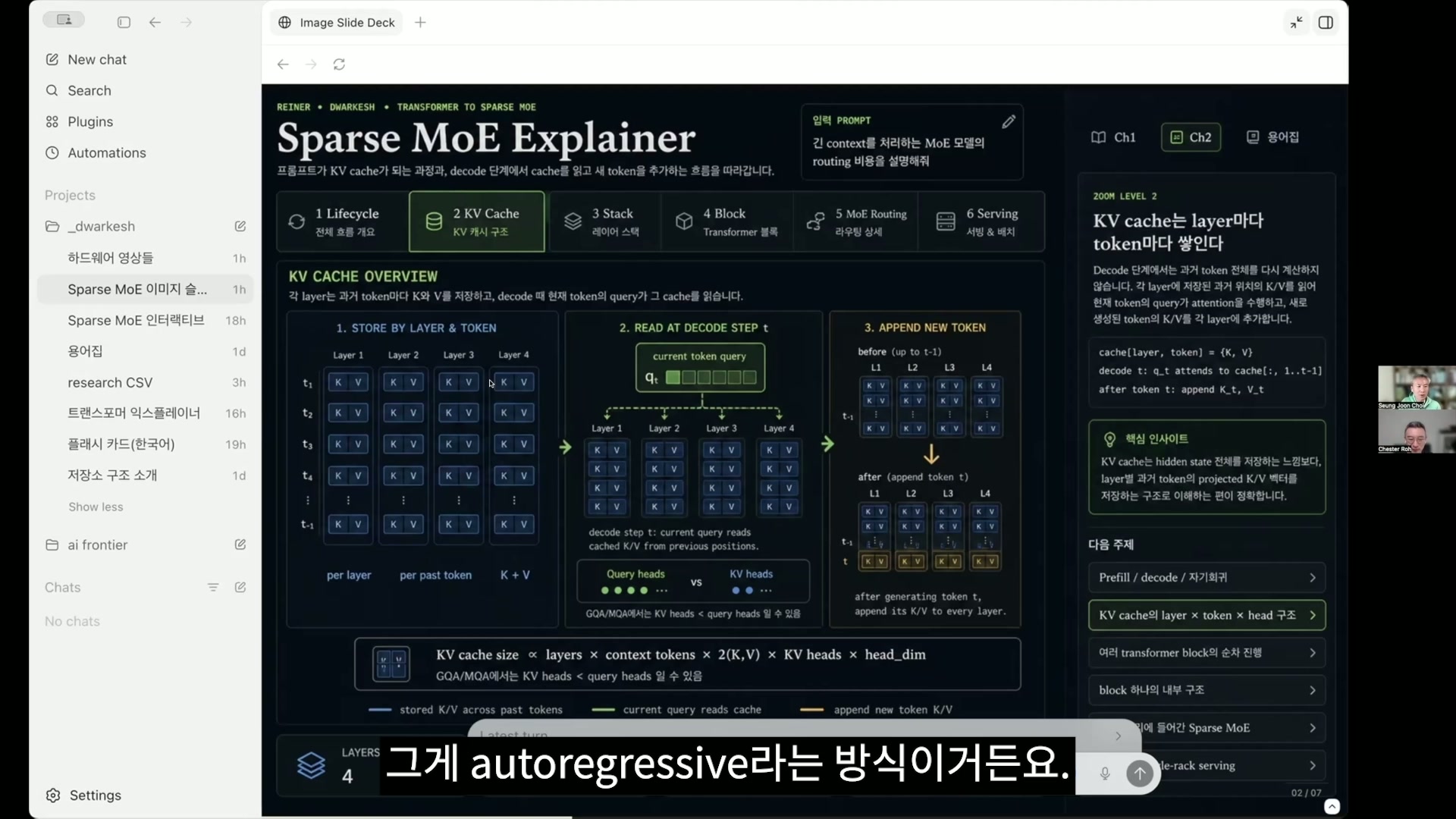
Inference terminology basics: KV cache, prefill, decode 9:19
Chester Roh Because hardware develops this way and models develop that way, hardware also turns in that direction, and because hardware is like that, models also change in order to fully utilize it. Today’s content is a bit difficult, isn’t it?
Seungjoon, while doing our episodes, we have actually tried many times to explain transformers in an easy way. But this really does not work well.
Always, what on earth HBM is, and then the basic structure of a transformer, within it, what this attention and fully connected layer, dense block mean, the story of KV cache, which is talked about in many places, but what exactly that thing is, and then what prefill and decode are, and what a forward pass is.
But the fortunate thing is that inference is easier than training anyway.
Seungjoon Choi We are not going to do training.
Chester Roh Take that one bit of comfort, and today, regarding inference, only up to the forward pass. The backward pass is actually about training, and now I do not even want to look at that. In all modern architectures, with these MoEs and sparse attentions laid out, how training would be done is something I now do not dare even try to open up, so let’s try explaining it at about this level. All right, then, Seungjoon, shall we talk about transformers just one more time?
Transformer execution flow and KV cache reuse 10:49
Seungjoon Choi I think we need to talk about it from the big structure.
We will go into detail here now, and when getting the overall picture, the reason we talk about this is, not only in IT but probably in other areas too, if there are resources, there is a tendency to extract as much from them as possible. They should not sit idle. So that kind of thing will come up later as well,
but first, I will talk a bit about transformers.
So overall, when we write some kind of prompt, that becomes what is called prefill, and it is all computed in parallel at once. When it is computed in parallel, KV caches are created. I will explain that in a little while. Once the KV caches are created here,
after that is done, from the vector connected to that token at the very end, the next token is inferred, and that goes back in as input, so the arrow here goes like this. It decodes. So the prefilled part
and then the stage where it is decoded one token at a time can be important to think of separately. So I think we really need to explain this very simply,
Chester Roh and honestly, if you understand the concepts of prefill and decode, you can graduate, to be frank. Is that so? No, I was saying that as a joke. From the perspective of a beginner hearing this for the first time,
if this concept clicks for you, then honestly, that means you’re doing very well. That’s what I wanted to say, and just to help with understanding, let me explain it one more time, and please comment on it, Seungjoon. In Claude Code, when we say, “Hey, take a look at this code,” and suddenly paste in a thousand lines of code,
Seungjoon Choi Right. It has to prefill. Exactly. That goes into the transformer,
Chester Roh and for this model to output the next token, it has to do some preparation first. Right. You can think of that preparation process as what we call prefill. And for the most part, you can roughly think of that prefill as being about long input tokens.
Seungjoon Choi And what the user inputs also gets prefilling. Since it’s the user prompt, it’s the same thing. That’s the input.
Chester Roh Right. Since it comes in long, input tokens always get prefilling. So they go in, and those tokens that get prefilling are processed token by token, and for each individual token, QKV is calculated once. But in QKV, Q is used once and then discarded, while for KV, as you go further back, the query tokens later on have to look at all the earlier KVs. So I think it would be right to think of it as storing each one of them.
We’ll look at it in more detail a bit later, but in what you just explained, a transformer has multiple blocks. I think DeepSeek V4 had about 61 of them.
Right. What we looked at last week was that, for each token at each of those, KV gets attached. So if the input was 100 characters, KV gets attached for all 100 characters in one layer, and then KV gets attached again in the next layer, so you can roughly think of that KV being attached 61 times for every one of those 100 characters. That’s right.
Seungjoon Choi It becomes an enormous amount.
Chester Roh We’ll talk about this while looking at the transformer block in a little bit too, but in fact, when a token is input, and this is the charm of the transformer, it simply passes through 61 repeated transformer blocks that all look the same. That’s what Seungjoon was just saying, and the output token is taken from the topmost block, and that gets converted back into a token. Right. It has to be returned from what was generated at the very end,
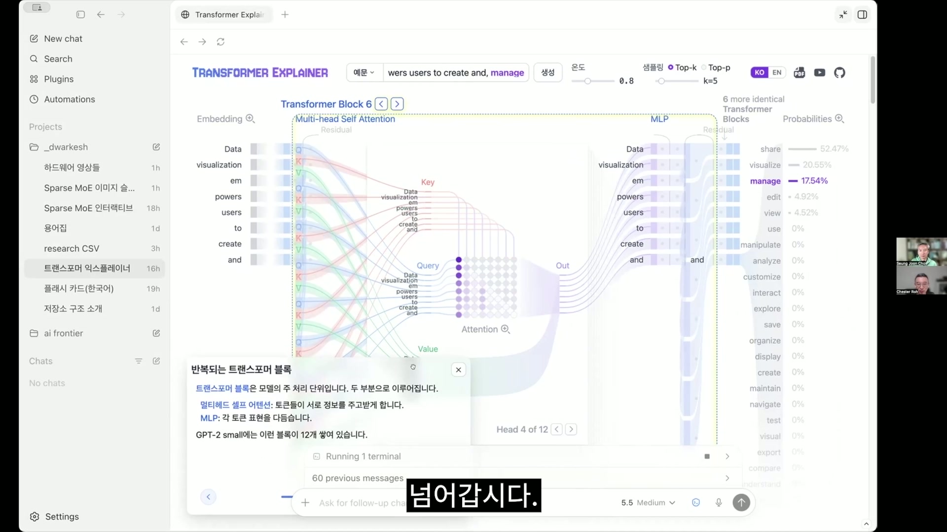
Seungjoon Choi and that’s the method called autoregressive. The details may take a bit of time, but this Transformer Explainer site is very well made. Compared to the version that views it in 3D, this explains it in a way that’s easier to understand, and GPT-2 actually runs here. I clicked around and made a Korean version of the explanation.
Chester Roh Oh, Codex did that for you. So this is what the transformer is about, and using GPT-2 Small,
Seungjoon Choi I’m going to show a bit of an example now. So if you look here, Q, K, and V are generated in various ways like this, attached as multi-heads even for a single token. But this is too detailed, so we’ll leave it at about this and move on. So, “Data Visualization Empowers Users to” But “Empowers” can be split into two tokens. Tokens and words are a bit different. We roughly lump them together and think of them as words, but Yes. Now, let’s follow this.
Tokenization: token IDs and vocab size concepts 15:29
Seungjoon Choi So what is the token most likely to come next? I’ll press generate according to the instructions. Then that gets calculated like this, and the word that comes after “create” is currently predicted as a comma. At 21.17%. So through this process,
the comma goes back in as input, and then the next one is generated. So if we generate again, “manage” came out. There are various candidates, and this keeps repeating after prefill. So the prefill just now was the process where QKV was calculated all at once like this. If we look a little more closely, here,
there’s something called embedding, where the token ID itself is fixed, and it performs the task of converting that into a vector. So in that kind of way,
Chester Roh What is a token ID? A token ID is, usually back in the GPT-3 era,
Seungjoon Choi there was a vocabulary dictionary of about 50,000 entries, and the actual tokenized word “Empowers” becomes two tokens. “em” has the ID 795, and this is fixed. “powers” is fixed as 30132, like this. The ID is fixed, so the same thing is always assigned at the beginning, but after it gets vectorized and flows through the internal residual stream, the context gets mixed in, so it changes.
Chester Roh Then we can think of that token as a kind of serial number attached to each word, and then what we commonly call vocab size is how many words are in this vocabulary that the model has, right? Right. But the important thing is that later on, too, we’ll mix up
Seungjoon Choi the terms token and hidden space when talking, but since the state is actually vectorized, we call this vector a hidden state, embedding, and various other terms interchangeably. But I’ll explain that again depending on the context. Anyway, for each of these tokens,
the important thing is that a vector is created. And positional is a bit difficult,
so moving past it quickly, anyway, it injects information related to position, The same Transformer block as Chester mentioned earlier, in the case of GPT-2, keeps appearing like this. So it is showing how many identical ones are left now.
And as it keeps passing through these, calculations proceed to derive which direction it should go in, and what direction the final output should take. And QKV is created in all those layers, and KV is kept. So it can be calculated again later. So if the query feels like a query made from these prompts,
Attention causal masks and KV compression techniques 18:29
Seungjoon Choi from the tokens, the key and value are actually from the knowledge. This is often explained with the concept of soft search. It is not exactly finding a key-value pair, but softly finding information, that kind of feeling. So as you look at this,
Chester Roh if you try to understand some meaning behind QKV, it gets difficult. This is something the authors of the Transformer, saying, “When these tokens come in, if we want them to calculate their relationships with each other inside, how should we do it?” just structurally created as a kind of bias. So when that token comes in,
it is split into query, key, and value and everything is calculated, and QKV is calculated in this kind of way. Of course, there is naturally a philosophical meaning to it.
But it is a kind of inductive bias made that way, and you can just think of it as the authors’ design. Please do not ask why, when this becomes like this,
it becomes a query, a key, and a value,
and let’s move on. But this animation is interesting, so let’s take a look. If we go into attention in detail, it calculates something for every token with every other token like that. And that creates contextual information. But the reason it forms a triangular shape here is when future things are input into the prompt, I’ll skip that. Explaining the causal mask is a bit difficult. Yes, let’s just move on. Naturally, it should only look at what came before.
Because the future token has not arrived yet. That triangular thing is just called a causal mask, and such a thing exists. The author made it well. But So things like that exist as multi-head,
Seungjoon Choi and the difference between old Transformers and modern Transformers is that in the past, if all of this KV was kept, these days, compressing it is also important, but that is for later, later.
Chester Roh Yes. There are a lot of tremendous techniques inside that, and recently,
Seungjoon Choi Things like MLA and sparse attention, all of that. Right.
Chester Roh I think DeepSeek V4, which we covered last week, showed the ultimate version of that, so let’s move on. Yes. Because it becomes too much.
MLP and MoE architecture: intuition for sparse MoE 21:06
Seungjoon Choi To store. And then next, this is the MLP part. After passing through attention, it is also called FFN, and also called MLP, and the hidden state goes through an MLP with a very small layer, usually about one hidden layer. Sometimes it can be one or two, so when that happens, there too, in terms of the general feeling,
some information is retrieved there by the vectors going in. If you look at it by the size of retrieval, the MLP has much larger weights than attention. So there is more of something here,
and this is the part connected to MoE. Yes. In the past, that MLP part was one large block,
Chester Roh and all of those things were calculated, which we described as dense. It was dense, meaning everything had to be calculated, but MoE split that up.
Seungjoon Choi So now, in the case of sparse MoE, when we covered DeepSeek V4 last week, something like 6 out of 384 were activated.
Chester Roh I forget the exact number, but it was actually a very large number, and it was very sparse. Yes.
Seungjoon Choi So that will come up as important several times today as well. In that way, among various candidates, as you see here, the concept of a logit appears, and a logit is ultimately what comes before turning it into a probability. So certain scores come out, and by turning those into probabilities, it determines what will become the token from a vocabulary of about 50,000 words. So at this point, it is made back into a token, not a vector, and that token, as an ID, goes back to the beginning and becomes a vector again. That is the autoregressive method. So what you put into the input, multiple words are processed at once,
Chester Roh but then the next-word prediction, just the next-word prediction, requires one thing before it to come out so it can be stacked on top of that and then request the next word again. And the good idea is that the previous KVs
Seungjoon Choi have already been calculated for all the earlier things. They can be reused. The query is created again for that one newly generated token, but the rest uses what was already there, and the KV of the newly generated token is merged into it. That is how it proceeds. I will skip top-k and top-p here. So this has been the Transformer very quickly.
Chester Roh Right. This is how a Transformer is structured. When words come in, the words are split and converted into things called tokens, and those just have labels like hello is number this, and something else is number that, as we perceive them. To put those labels into the model, something like position is also added, and through embedding, they are converted into vectors that it can understand. The words are. And now,
that is actually what we call tokens, and they go in, pass through attention, and inside the attention block, there is an important concept called KV cache, and after coming out of that attention block, they go into the MLP block again, are computed, and come out. Yes. And what comes out goes around like this,
Seungjoon Choi but one important thing we left out is the concept of the residual stream. I should have talked about it, but when each one comes out, it adds to itself and gradually updates its meaning. Yes. That is actually a very important part.
Chester Roh It’s an important concept.
Seungjoon Choi So in this way, a residual stream is created each time. For all the vectors, for the tokens that have become vectors, it adds the attention information to itself, then combines the MLP result with itself, and keeps chaining that through every block. Yes, that’s right.
This is actually an important part where an important flow is created. Right. In the diagram you see here, there are blocks 1, 2, 3, 4, 5, and n,
Chester Roh and in the case of DeepSeek, it has 61 blocks.
Seungjoon Choi GPT-3 actually had even more. It had around 90. I see. And the things that exist inside those blocks
Chester Roh are the attention and MLP blocks, and those two are the core parts. And in the architectures of the various latest models we’re looking at these days, most of the changes are about how to make the attention inside them use less memory and compute faster, and then how to make the dense block smaller and make computation more efficient there. That’s right. So I didn’t explain the LM head here,
Seungjoon Choi but in any case, the LM head comes at the very end, after computing many things, and for the final token, meaning only for this vector, it is used to infer the next thing, to predict what the next token will be. And that, along with the next slide, is probably a diagrammatic representation of the mechanism you mentioned earlier. The parts with plus signs are where the residual is combined.
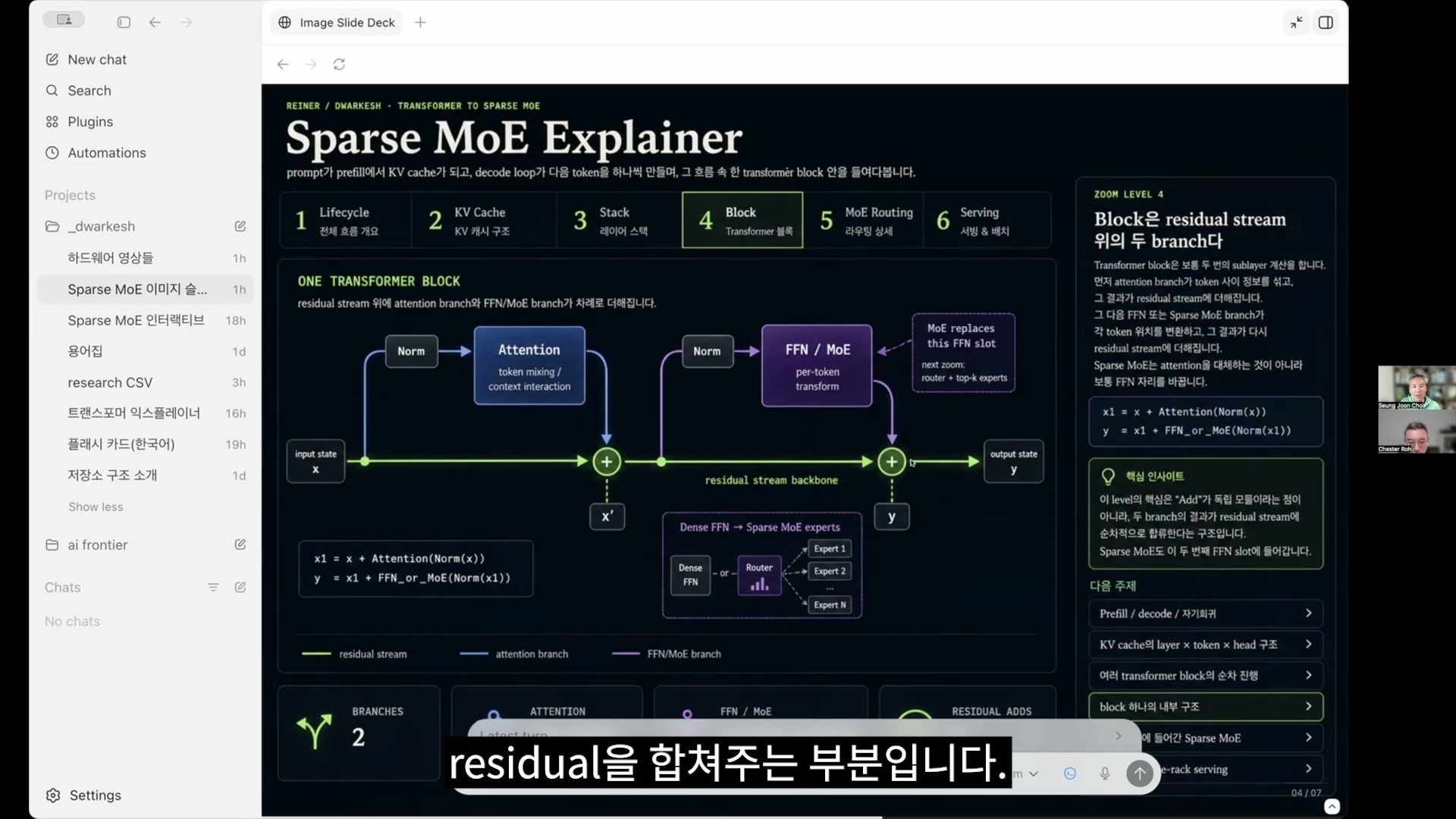
Chester Roh The green line below is the residual connection.
Seungjoon Choi It’s making a residual connection.
Chester Roh This is showing one transformer block right now.
Seungjoon Choi That’s right. So one block can be diagrammed like this. But here, what was just shown as FFN or MLP, and then MoE,
these days, since parameters have to be increased, if you want to make it large enough to fit in memory, the problem is that you have to split it up. This is one of today’s key points, and I made an interactive version of that. So for each token or vector, only part of the MoE is activated.
So at first, for example, if only one is turned on, here I have made only two, unlike the real case, out of the total 16 MoEs, connect to it. For this, two particular FFNs or MLPs are made to operate.
And then a weighted sum is taken and connected to the next stage. If you do this once, it becomes four. But sometimes,
there are cases where it is not doubled. Up to now, everything was doubled, and now 1, 2, 3, 4, 5, 6, 8. It was doubled.
Let’s look at another route. So this time it is 1, 2, 3, 4, 5, 6, 7. Since there are seven,
you might expect it to become eight, but it becomes seven because one expert… An expert did it twice.
Chester Roh Here, this is called MoE, Mixture of Experts, and the part many people get confused about is that because the concept of an expert means a specialist, they think if I ask about math, math is handled by some expert, and if I ask about physics, some other expert handles that, so experts must be separate units containing different kinds of knowledge. Some people think that, but that is not the case. Even if you type “I am a boy,” each of those may pass through a different expert.
Seungjoon Choi And for each token, as mentioned earlier, it passes through a different expert. It’s just that they get grouped that way.
Chester Roh So if you ask why that happens, we don’t know either.
Seungjoon Choi And there are multiple experts in each transformer block. Hundreds of them. So that part is important as well. So lastly, the hardware structure for
In-rack communication (NVLink, NVSwitch) and inter-rack bottlenecks 28:43
Seungjoon Choi how these things are served. Usually it is called a data server rack. We’ll look at a video shortly showing what a rack looks like.
There are multiple GPUs inside it, and inside one GPU, it seems good to group about two MoEs together. Looking at how it is done these days, when that happens, they all need to be connected to each other so computation can be done quickly. Computation within this is very fast through things like NVLink,
and these days there is also something called NVSwitch. It is fast, but between racks, this seems to take longer and becomes farther away, in terms of hardware. In a little while, we will look at the concept of racks,
Chester Roh but in fact, inside a rack, communication between GPUs is fast, and once it goes outside the rack, it becomes slower, so processing inside the fastest network is definitely the answer.
Seungjoon Choi And what gets transferred between these GPUs is ultimately something like tensors. Activated things and things like that are transferred to each other, but there is a problem where they have to be connected to each other simultaneously like this, so I think that kind of architecture is necessary. Then first, if we look at the video for NVL72, which was briefly mentioned earlier, it is about a two-minute video. Yes, it shows how our machine is made.
NVL72 rack configuration: a datacenter tour video 30:00
Chester Roh One Blackwell GPU is made by combining these two dies. The numbers will go by quickly.
Seungjoon Choi The yellow parts attached there are HBM. That’s HBM memory. And one was attached to the two.
Chester Roh Two GPUs and one CPU.
Seungjoon Choi It’s called a superchip.
Chester Roh And the CPU and GPU are also connected very fast.
Seungjoon Choi So this becomes one slot.
Chester Roh Then one slot has 4 GPUs and 2 CPUs.
Seungjoon Choi So it is one CPU for two Blackwells.
Chester Roh Just now, the interface card for communication goes in, so when you add this up, you can stack 72 of them.
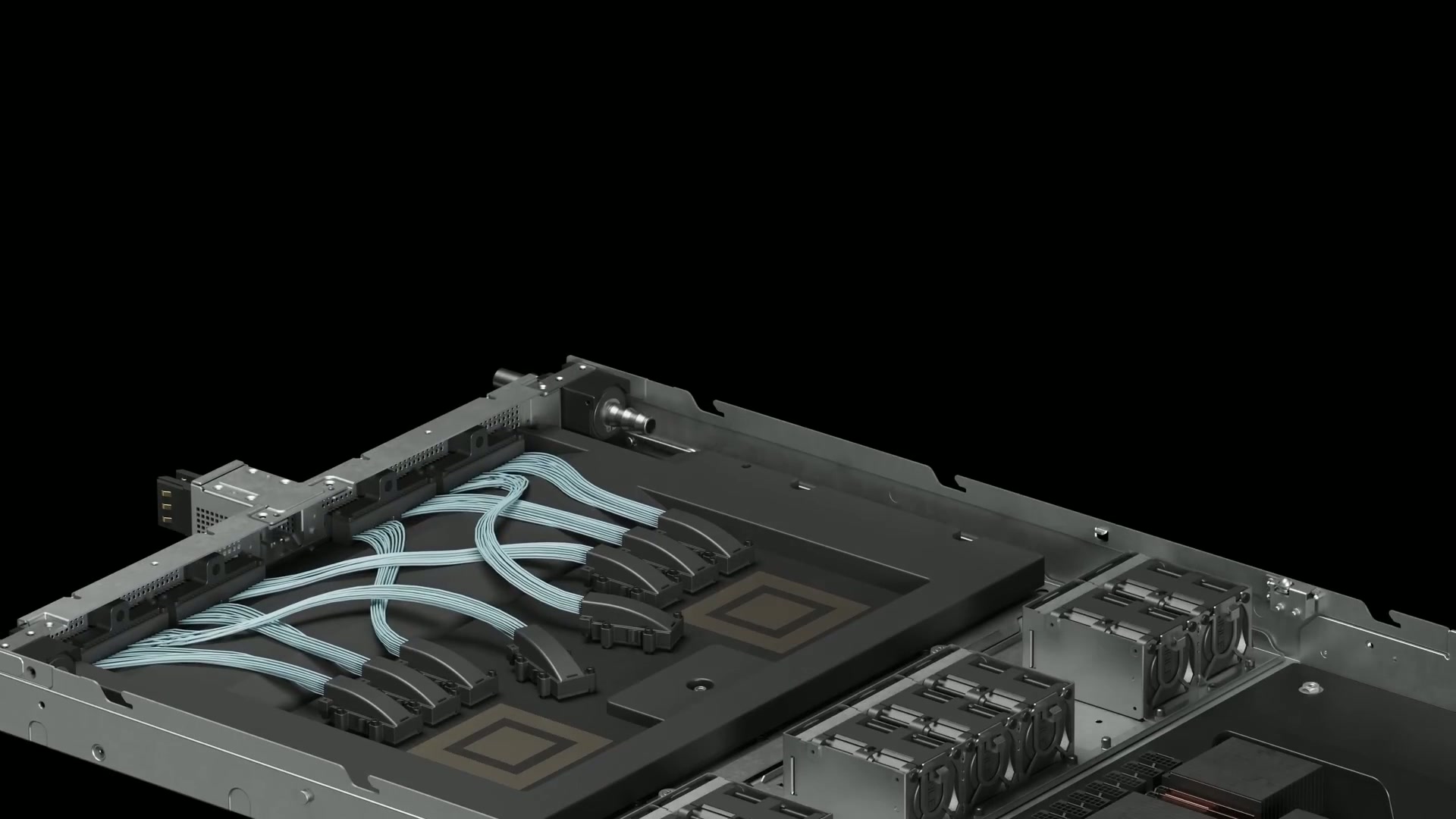
Seungjoon Choi And this is the switch, the one we saw in the diagram earlier. You plug that into the spine, and in the end, I think it is about what kind of highway you can lay down. Physically. So here, one rack, 72 of them,
Chester Roh with 72 GPUs inside.
Seungjoon Choi But there is something called InfiniBand. For things that require large bandwidth, to connect between racks like earlier, I think this is also called a DC switch. And that is the cooling pipeline. Liquid-cooled. So an AI factory data center
would probably cost an enormous amount like this, but you can build one. They showed this in the Blackwell era, and what they show in the Rubin era goes up one more level.
Chester Roh Yes. So there is one more video, and this one walks through how this has developed at this year’s GTC.
Video On April 6th, 2016, a decade ago, we introduced DGX-1. It gives a rundown.
Seungjoon Choi It comes up at about 1 hour and 7 minutes into GTC. So I think you can watch that. So, where this has come to these days, things like that.
Jensen Huang Hot water, 45 degrees, which takes the pressure off of the data center, takes all of that cost, all of that energy.
Seungjoon Choi This much is also 72 now.
Jensen Huang They use LPDDR5, LPDDR5 and incredible single thread performance.
Seungjoon Choi Now Jensen Huang cannot lift it up and show it anymore. That’s it. We built
Jensen Huang that so that it could go along with the rest of these racks for agentic processing. Up to here is Blackwell.
Seungjoon Choi So this is how NVLink is operated. So after watching this Dwarkesh video, I ended up looking back at Jensen Huang’s keynote again. Right.
Chester Roh Now, Seungjoon, since we have covered some of the background explanation, let’s start today’s main content. The content we studied for three days is a lecture Dwarkesh gave with someone named Reiner Pope.
Breaking down LLM serving time with roofline analysis 33:31
Chester Roh It is a session that helps us read how these GPUs are served, and what meanings are hidden in a few numbers, using simple formulas. Let’s follow this session together and go over the meanings.
The discussion proceeds by saying that they will do roofline analysis. What this person is saying is that in the end, when we write something in Codex or Claude Code or ChatGPT and press Enter, there is a time it takes for the result to come back. But that result does not just come out
all at once like a page of A4 paper;
we see the tokens being generated, don’t we? We see the decode process. Right. That process is very fast for some things
and slow for others, and of course now everything has leveled up quite a lot, but in the past we often saw cases where it was slow, didn’t we?
Seungjoon Choi That’s right. And the time until the first token appears is also subtly different, isn’t it? Right. So this explains the concept
Chester Roh of what on earth is happening inside in those cases. But this is hard to just skip over and only talk about the conclusion, because unless we follow some of the intermediate content, there are parts that are difficult, so we will follow it step by step too. Sounds good. Here, t is time.
Latency determined by t_mem and t_compute 35:12
Chester Roh In other words, the time it takes, the time it takes for an LLM to produce some result, is described with these two things, T_mem and T_compute. So memory time and compute time, and it is limited by whichever of the two takes longer, bound by it, is what I think they are saying here. Right. And so, what is the time compute takes? That is what they are asking.
Seungjoon Choi The term active parameters came up. The time taken for this compute
Chester Roh is actually what we just talked about in the transformer. The main components that take time in computing are actually the attention calculation part and then the dense block behind it, which is called the MLP block, multi-layer perceptron, the kind of neural network we are traditionally familiar with. The naming is confusing.
Seungjoon Choi Sometimes it is called MLP and sometimes FFN, but they are talking about the same thing.
Chester Roh Right. They are talking about the same thing.
Right. They are talking about the same thing. Here, they mean the expert. Right. But now those two blocks are the sum of the time it takes to compute them.
Right. But here, when calculating T_compute, they only calculated that dense block. For the sake of calculation, what is the time taken for compute here, actually? It is the number of these parameters multiplied by the number of tokens we put in, isn’t it? Right. The tokens we put in are processed as a batch, but we should actually explain the concept of this thing called a batch before moving on. So,
Inference batching concepts and scheduling/orchestration 36:46
Seungjoon Choi Couldn’t you see it as similar to sequence length? Though maybe it is sequence length used by multiple people.
Chester Roh So here, I think we need to distinguish a little between batch in training and batch in inference. So batch in training means we use the term batch to calculate multiple sentences at once, right?
Seungjoon Choi Right. We do that to run GPQA all at once. To run it all at once. So when there is a batch,
Chester Roh the sequence length in one batch is usually within the range that training allows, for example 4K or 8K, and the sequence length is fully filled across that range. Right. So usually when training, If you look at the dimensions of the tensor we put something into, it’s batch, then sequence length, then embedding, the product of these three things, which we call the hidden dimension.
Seungjoon Choi d_model. Right. That one is full.
Chester Roh So batch times some sequence length effectively becomes the size of the dataset, but in the case of inference, the problem becomes a little different. How does it change?
Seungjoon Choi Depending on what input you give, the generated length is different, the input is different, everything is different, isn’t it? That’s right. But when we do prefill,
Chester Roh multiple tokens go in at once, so if things line up, it can become similar to training, but in the case of decode, this one previous token has to come in before the next token can advance. So in reality, the number of input tokens is only one.
In other words, the sequence length is only one.
So from a traditional training perspective, if we assume a batch is one user, one user might write a sentence like “Hi,” while another user might just throw a 50K context into Codex, and another user might just have one paragraph. In reality, the length varies too much. If we had to fill
those same dimensions as in training, wouldn’t we have to push the other parts with padding? Nothing is in there. It’s sitting idle. Right. Then that becomes an enormous waste of memory,
so the reasonable idea is to remove all the padding and just concatenate everything, isn’t it?
Right. That is actually the concept of batch in inference. That’s right. If you concatenate these, there are parts that get completely messed up,
dimensions, KV, and things like that all break down. That’s actually right. During training, within one batch,
according to the sequence length laid out in it, the KV is exactly aligned, but during inference, if you just put the single-token pieces from multiple users into one batch, all the tokens needed to move to the next token, doesn’t the entire KV cache get messed up?
Seungjoon Choi I don’t know the details either. Since this gets messed up,
Chester Roh in practice, systems like vLLM or SGLang put in a meta layer and match everything up. So if we just look at the conclusion, inference also ends up being that one batch, on the one GPU we are using right now, as if thousands of people are connected to it at the same time.
Seungjoon Choi Then there has to be a scheduler for that. Yes, there is a scheduler.
Chester Roh There is a scheduler and a meta layer, so it says things like, “In this batch, the 100th item belongs to user Seungjoon, the token at 103 belongs to Chester, this token belongs to this person,” and it keeps all the indices for those tokens. Then after it goes through the transformer block and comes out through computation, all the KV operations have to be done in between, right? Right. But each user’s situation will also be different.
One user might already have used something like an 800,000-token context in front, while another user might have zero context.
Seungjoon Choi There must be many cases where the cache has been wiped, yes. There are also cases where it gets compacted and wiped.
Chester Roh But in the end, that preceding context is the KV cache chunk we talked about earlier, so all the metadata that maps those KV cache chunks runs. You can assume that the meta layer, the orchestration layer, is all running.
So the dimensions in inference and training are a bit different, and the batch that people familiar with training think of and the batch that Dwarkesh is talking about today, the batch in inference, are different, I think we need to say that. The reason for doing it that way is important.
In a sense, the reason for doing it this way may be the most important part.
Difference between GPU utilization and MFU 41:36
Seungjoon Choi Because you can’t let an enormous GPU sit idle. Because it’s an expensive resource, it must not sit idle.
Chester Roh Since it must not sit idle, every time this one step runs, you have to run it packed full. So GPU utilization has to be around 70 to 80% for this to be a profitable business. Is that what MFU is?
Seungjoon Choi Model FLOPs Utilization, isn’t that related?
Chester Roh I think MFU and GPU utilization should be seen as somewhat different concepts. MFU is about FLOPs, so for this GPU, assuming it is running at full capacity,
Seungjoon Choi When the output is at its maximum.
Chester Roh Yes. Without accounting for memory bottlenecks and things like that, if you just compute optimally, it calculates 100, but in real-world computation, that doesn’t happen. You have to wait until the data is ready, and do various other things, and because there are so many things that block, in reality many operations are not compute-bound, but are often memory-bound, so you cannot use all of the MFU. But after accounting for MFU, I/O, and things like that,
the concept that if the GPU is running, then it counts as running seems to be GPU utilization.
So in training or inference, raising the MFU number is always good. And this person talks about this a bit later, saying that the point where MFU is maximized is just when T_compute and T_memory are equal, and then just glosses over it.
Seungjoon Choi For now, something like the intersection point where they meet. So I explained it verbally,
Chester Roh but at least for transformer training, the B and N we talked about earlier, and then the model dimension, this concept of the tensor, if that is not firmly fixed in your head, then honestly, it is a little hard to keep understanding this, so you can just move on thinking, “I guess that’s how it is.” But in inference,
batch and sequence are just flattened into one, and that is treated as one train, with multiple users’ workloads riding on that train at the same time. So when one clock cycle goes around,
to carry as many users as possible. But on that train, there are all kinds of different passengers. For example, if that user
is simply in decode, assuming everyone is in the decode process, then there will actually be only one token going in as input, so if, for example, the batch is 2,000, you could carry 2,000 people at the same time. Right. If we just, to put it roughly,
Seungjoon Choi the model has to keep doing matrix multiplications with those weights, and it feels like filling what gets multiplied in that matrix with the passengers’ data. It has to do that all at once, and keep doing that every 20 ms or whatever, repeatedly, so it feels like the train keeps departing.
Chester Roh You just set one clock at 20 ms, and since that comes up again later, let’s talk then about why it is 20 ms. In the end, you are filling the train,
and to wrap up what we were saying earlier, if only one token goes in at a time, then 2,000 people could use it simultaneously, but if, for example, someone dumps a huge amount of code into Claude Code, and there are about 1,000 tokens that need to be prefilling, then in practice those 1,000 fill up as prefill, and then the users doing decode fill up about another 1,000 behind them.
So how to optimize this process of prefill and decode is really the core of modern LLM serving these days.
What is the goal? Ultimately, per unit time, memory or compute,
you have to maximize all of it. Utilization. Everything is centered on
how to use this as fully as possible. Good. Then let’s leave it at that, and as more concepts come up later,
we can go through them one by one.
So T_compute is basically saying this.
Batch, how many people will you carry?
For convenience, let’s say it is one token.
Then if you carry 2,000 people, B is 2,000.
And N_active is just the number of parameters that are activated.
Now this person brings in the MoE concept here, and the idea of sparsity is that the total parameters are this much, but the core idea of MoE is that when computing, only a few experts are computed quickly.
That is why efficiency arises in computing.
Seungjoon Choi It is also a way to increase the total size of the parameters, and it is also about efficiency, things like that.
Chester Roh Right. So for that efficiency, T_compute is batch multiplied by this number of parameters, bounded by the number of active parameters, and this expression is used to represent that. If you divide that by FLOPs, how many computations can be done per second, you get the unit time it takes. Right? For the denominator below, if we just roughly treat it
Seungjoon Choi as computing power,
Chester Roh That is the assumption.
Seungjoon Choi then it would come out like this. Yes, it does.
Chester Roh So of course, attention is missing here, and this person is saying that, for convenience, he will leave it this way for the concept of computation. But when attention goes into the sequence length, if that context length gets larger, the attention cost actually rises, and if it gets smaller, it decreases. But this is actually an important point, so I think I should mention it before moving on.
In practice, even when this is long, they do split it up and put it in. For example, the code we need to put in,
the code sent from Claude Code, even if it is something like 50,000 tokens, they do not put all 50,000 tokens in at the same time. They split that up again, say into chunks of 1,000, and mix them with other people’s decode tokens to carry them together.
Seungjoon Choi So the point is to fill it somehow. Right. Fill it somehow.
Chester Roh And Dwarkesh asks about exactly those kinds of things. Since we have already covered almost all of this, we will now just move on to the memory side. So this formula,
Seungjoon Choi it seems like he is writing the one for decoding now. Yes.
Chester Roh Yes, he writes it out while talking about decoding, but I think for us now, it is right to look directly at the calculation with this in front of us. Then how is memory time determined? First is N_total, and actually, here it is total. Because you have to hold all of this. When computing, you have to load the entire model weights into memory and keep them there. And in the case of experts, since you only need to compute the experts that are activated, compute used active for this. Right. When computing,
Full memory-time model: full loading and KV cache costs 48:16
Seungjoon Choi you can just pull in and use the weights for the active ones, but for the memory calculation, you have to hold all of them.
Chester Roh Right. But for the memory calculation, since you have to hold all of them, that is why it is N_total, and then plus, here, actually, attention was omitted above, but here he puts it in. Batch, and then each batch has a different length. If the context is decode, it will be 1, and if someone is in the process of doing prefill, this becomes quite long, depending on that, and here, if you multiply by how many bytes are needed per token, this comes out. Right. Here too, actually, briefly,
Seungjoon Choi What confuses me is, when it is decode, is it 1? In the end, it’s the prefilled part from before plus one at a time as it keeps going. Because it’s the length. No. That’s not how it is, because that part is something Seungjoon understandably gets confused about a lot,
Chester Roh but actually, the token that goes in during decode is the last token output from the previous step, meaning the immediately preceding step. Only that one token goes in as input.
Seungjoon Choi Because the KV from before is already there.
Chester Roh Right. So it goes in as input, and in effect, the tensor that follows this flow through the transformer block is just that one input token.
But even though only that one input token goes in, in each transformer block, whether it was prefilled earlier or came from an earlier decode step, the KV cache blocks for the prior context will all exist for each block. Right. They’re all there. That’s what gets loaded from the cache. If that’s in HBM, it happens quickly,
and if it’s not in HBM, it has to go somewhere else and fetch it, but in any case, somehow it has to be loaded into HBM for the computation to happen. Since that computation is what it’s doing,
actually, as I mentioned earlier, in this one inference batch you can pack in a very large number of users together. Because in the case of decode, only one input token passes through.
Seungjoon Choi Right. So they would be mixed together like that.
Chester Roh So this is where it gets complicated, but the users’ KV caches will all have different lengths. Some are long, some are short, and so on. Since the KV cache disappears over time,
Seungjoon Choi it could also rebuild everything from scratch with prefill, going back over all the earlier input.
Chester Roh Right. If the cache doesn’t hit, say I type something, hit Enter, then suddenly someone calls me from the side, I go eat, and come back an hour later, then in effect it’s all gone from the cache. In that case, it’s actually prefill again. Right. It has to run the prefill loop again from the very beginning and build the KV cache, so the price of the input tokens gets calculated again then, which is expensive.
Seungjoon Choi Right. It becomes expensive. But if it’s loaded from the cache,
Chester Roh if the cache hits, you can get it cheaply, so it becomes cheaper, and those are the economics of inference. But going back to the KV cache as I mentioned earlier, if you imagine putting many users’ single decode tokens into one batch and computing that cycle upward, the lengths of the KV caches will all differ by user.
Seungjoon Choi Of course. The innovation called PagedAttention,
PagedAttention and making KV cache memory-efficient 52:12
Chester Roh which vLLM created, is essentially what made it possible to optimize those differences extremely well and pack them into one memory block. If PagedAttention had not existed,
we would have had to put users’ KV caches into very static tensors like we do in training, and fill the empty parts with padding, which would have wasted a lot of memory. Instead of doing that, it divides things into block units, as if we were using pointers to mark exactly where all those KV caches are. So as that computation goes upward,
it finds the pages in the KV cache and computes all these tokens. How to take things like this
and turn all of them into one vectorized operation is, honestly, almost everything in this inference process.
So I’ll keep talking about this throughout the conversation, but what is the purpose of doing this?
You can think of all these considerations as being there simply to maximize GPU utilization. In other words, if you don’t take one GPU and maximize its utilization within a fixed amount of time so that it can serve 2,000 people at the same time, we wouldn’t be able to use this for $20 each. Another thing I’m getting curious about, and I’m sure it will come up later,
Seungjoon Choi is that right now, memory, meaning HBM anyway, is being used for the model weights and also for the KV cache, right? These days, where is more of it used?
Chester Roh We need some arithmetic here too. For example, the latest GB300 connected as an NVL72 rack that we looked at earlier, one rack has
Allocating model weights vs. KV cache within 20TB HBM 54:03
Seungjoon Choi About 2 TB?
About 2 TB? No. 20.
- Right. 20 TB for one. Right. The HBM inside one rack is about 20 TB,
Chester Roh and the CPUs there also have LPDDR5 all connected to them. And that memory is also about 20 TB.
So in total… For the CPU? For the CPU.
What we commonly know as RAM, that’s 20 TB, so in total it has about 40 TB of memory, and I’m not sure whether there is SSD storage inside.
Anyway, storage too… Right. That has to be offloaded. It must be there. Let’s assume it is. But when calculating,
people usually don’t include storage.
Seungjoon Choi There was something called Blue something. I forgot, though. (NVIDIA BlueField) If we look at it that way, there is about 40 TB of memory,
Chester Roh but we usually load all our weights into HBM. So we can assume that the 20 TB is essentially there for us to do deep learning computation.
Seungjoon Choi Then if you just think of the model as FP8, just as bytes, isn’t there a lot of room these days?
Chester Roh Right. Yes. A 5T model is 5 TB.
If you calculate a 5T model in FP8, as Seungjoon said, just fully loading that model takes up 5 TB of capacity. Right. Then the remaining 15 TB is left. So many people
also get confused at this point and say, then can’t we just load four models into it? But no.
In reality, you also need capacity for the input coming in, and every time that input goes through a transformer block, for the attention computation, you actually need memory for all those activation parts. For the intermediate computation, you need those intermediate results, and you also need to store those activated values. Most of all, the biggest thing is the KV cache.
Whether the context is long or short, you have to hold every user’s KV cache, so the KV cache takes up a huge amount, but this depends on how you allocate it. Here, it really comes down to what batch you will take, and what context length you will allow for users. Those are what determine the number of KV caches, after all.
So there is a bit of a trade-off among those things, but if you have around 20 TB of memory, you allocate 5 TB to the model, and actually, it could be even smaller than that. These days, people reduce it a lot more with FP4. So out of 20 TB,
they allocate about 13 or 14 TB to the KV cache. And about 2 TB goes to the activation variables computed in the middle.
But since those variables can keep being overwritten, you don’t need to keep that many of them.
Seungjoon Choi I think we may have jumped ahead in the discussion a bit, but anyway, assuming a 5T model, although assuming a 5T model is already the issue here. In reality, what we know right now was serving for models of around 1T to 2T, and because NVL72 came out, we were estimating that it became possible to serve something around 5T.
Chester Roh Right. In practice, even if the training process is not this, there are many ways to do it, so even on an H100 or H200 cluster, if you wanted to train a 5T model, there are of course ways to train it. But in reality, these large models on H100 or H200, where the memory is small, and where inter-GPU communication like NVLink is very limited, the number of nodes… Even up to 2023, it was eight as one unit.
Seungjoon Choi Was it 2022 or 2023? Anyway, I think it was around then.
Chester Roh Wouldn’t it have been until early 2025? Before NVL72 came out.
Seungjoon Choi Before it came out, it was eight.
Chester Roh It was eight. But it has not been long since NVL72 came out, actually.
Seungjoon Choi It was late 2024. Right. We are a bit weak on these release timings, numbers,
Chester Roh and architecture. If CEO Jeongkyu were here, Jeongkyu would have explained it all clearly here, but right now the two of us are studying through it with difficulty, so for today, we will just move on.
So in the end, the point Seungjoon made is correct. Because it became NVL72, in the most current, modern inference environment, there is an enormous benefit. I think that is about how we can put it. We were talking about memory, and then the story suddenly jumped over here, but to summarize these two equations again, you have to understand this for all the following things to make sense. So of course you understood this, right? We understood compute,
Latency graphs by batch size and the concept of amortization 59:07
Chester Roh and memory is the time for loading total memory, and then here, the time it takes to load the context, and those added together are divided by memory bandwidth. In the end, memory also takes time to fetch all of this.
Seungjoon Choi The reason the denominator kind of has a time term throughout is that this is calculating t. Earlier, FLOPs were about how many floating point operations you compute per second, and now, too, because bandwidth is in bytes per second, in the end,
Chester Roh the hidden seconds
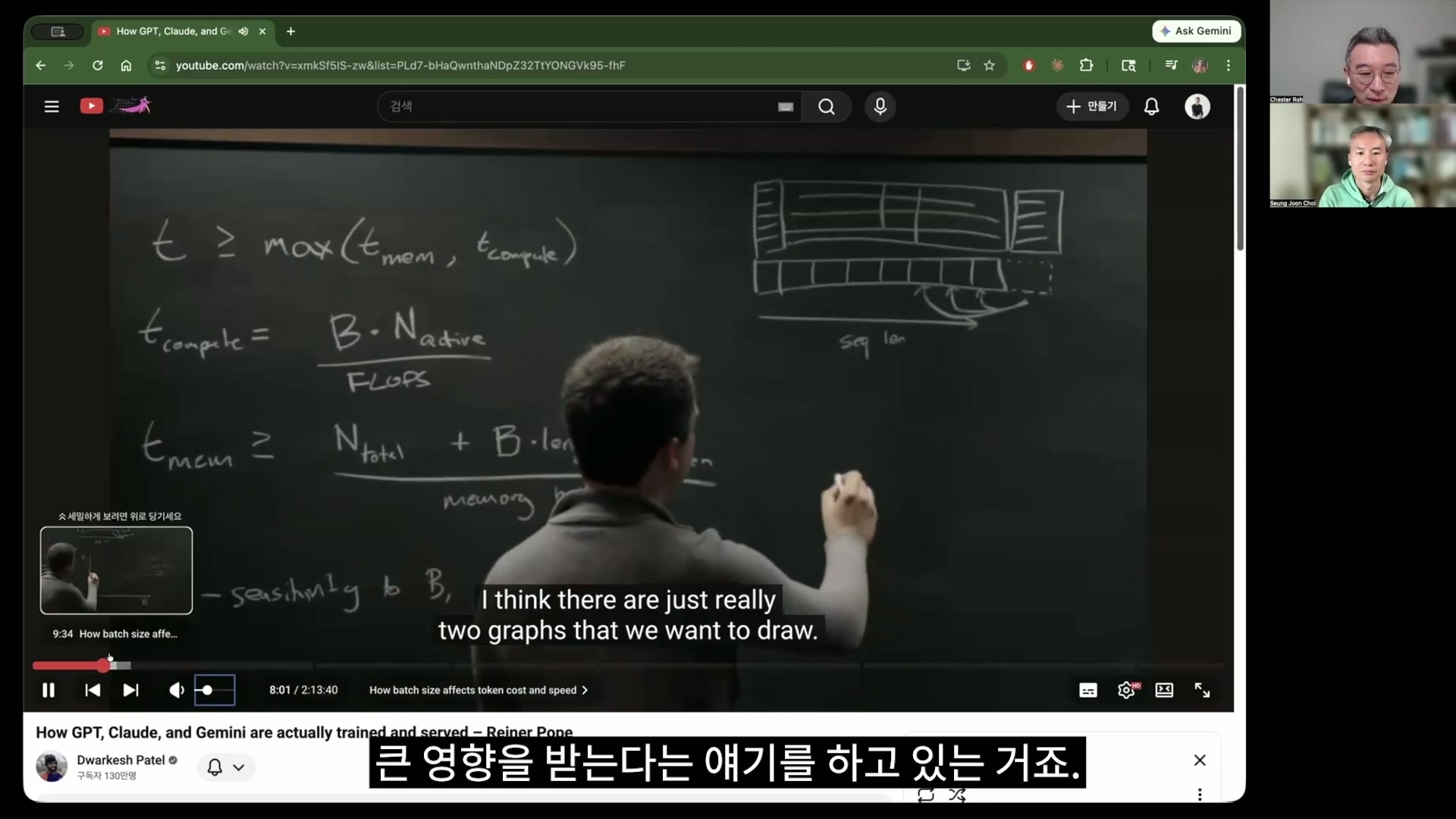
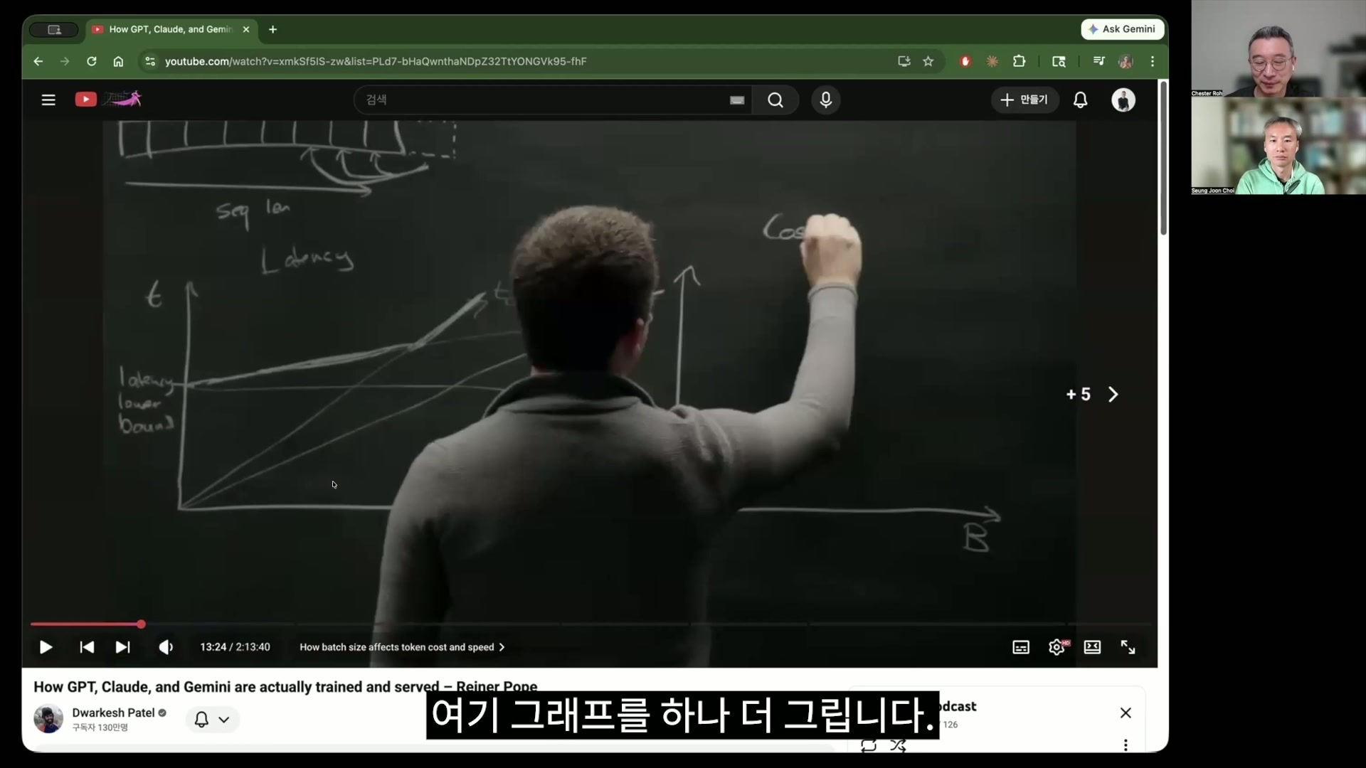
Seungjoon Choi come up as t. Right. It’s arithmetic. So the key things above and below are all capacities. That is why seconds come out in the end. So with these two, we are going to look at where exactly time is spent in modern LLM inference. So what this is saying is that this and t_memory are greatly affected by batch and context length. Shall we move on now? So this graph, I will turn off the subtitles for a moment. Drawing this graph is very important for understanding today’s topic. On the x-axis on the right is batch, meaning how many users you process per time unit, this batch size, and the time it takes because of that. This is plotting that function. And using these terms in front, we do the arithmetic. t_compute will actually be a linear function of batch here, so it is drawn linearly like this. Then for this memory time, the time to load total memory is just loaded once, and after that you can keep fetching and using it, so there is one very big intuition here. Once you load this memory, the longer you use it, the more you can offset the cost that went into it, so in this expression, they call it amortize, borrowing the accounting term for amortization, and they talk about that a lot. Amortize came up several times. And then the next graph to draw is the time to fetch this KV cache. But as the batch for the KV cache gets longer and longer, naturally, the time to load the KV cache will get longer, so why is this drawn below compute, then? That’s just this person’s choice. They are saying roughly that this cache time will increase by about this much. But N_total and N_active are different here, though they are just lumping them together. Right. They are lumping them together. But in compute, actually, N_total does not have an effect. Because N_total is a memory-side variable; when computing, that total memory has on the computing time has no effect at all. Because we only compute the active ones, so that’s how you can take it. Then here, let’s make this gentleman’s graph we just saw easier to see. Since that was also addition, not multiplication, anyway. Right. But here, Seungjoon, before we move on, what we saw earlier in the DeepSeek discussion has a big effect here. This KV cache time and this T_compute time, these two linear graphs. Right. With the slope of this graph, in fact, we explain all of time and cost. But the issue is that DeepSeek pulled this one way down. By lowering this, all the frontier curves come down. Then the intersection point also comes down, so now we end up talking about that. So that is what we now end up talking about. So this blue compute graph came from compute earlier, and this linear function for the KV cache and simply loading the total parameters, it will now add these two together. At the level of common sense, I also don’t know hardware well, but no matter how fast HBM is, it is not on-chip; it is next to the GPU. So it takes time. It would. So those things are now going into the cost. There are so many things tangled together, and for me, this session was good because it sparks the connection between what this hardware looks like and where it actually meshes with the algorithm running in practice. Then, coming back to this graph, it is difficult, even though it is just arithmetic. So the T_compute and T_mem we just drew are what this diagram plots on the graph here, and this slightly pink graph we just drew is the KV cache and then this time for loading the total parameters, simply added together. If you add the two, what we learned in middle school will come out. This is what comes out. In effect, this is T_mem. And in the end, we saw T_mem at the very beginning. What is the total time we perceive? It is bounded here. It is bounded by the max of these two, that is what comes out. But that bent part is where B is connected, right now. Right. Depending on what happens to that bent part, it will all change according to the hardware specs or the model shape and so on. Then what we did at the very beginning was to put down a max function and say it is bounded by whichever of the two is larger. Being bounded by T_compute and being bounded by T_mem, it is bounded by whichever of the two is larger, and now that is determined by B. So we are doing this to say that choosing the optimal B point well has meaning, and if you look here, this is it. When the batch is small, it is memory-bound, right. When the batch gets larger, it becomes compute-bound, that intuition comes out. The meaning. So now this is, in effect, T, so what is T? It refers to latency. In other words, how much we have to wait. So even if you start some small task here, the time to load all these weights is required by default, so this is called the latency lower bound. So we call it latency, use the expression latency lower bound like this, and this graph is a latency graph. We draw one more. The explanations we just gave are explained here. For those curious about latency, the explanations we gave in between are this. As if it were the conversation Seungjoon and I just had, if what in attention decreases, does that decrease or increase this, we talked about things like that, and here we draw one more graph. Cost, it is the cost per token. But it is this. This one went in as division. Right. In the end, this is the total time divided by the batch, so it represents how much was processed, how much was processed per unit time. Then for this too, B, we leave the x-axis as is and only change the y of this graph again. It is arithmetic, it is arithmetic, but you have to follow this content well. Earlier, T_compute was just a graph that increases linearly, so here it will just be a straight line, because we divided it. This may not make sense. For people seeing it for the first time, from batch to T to latency, there are probably many people for whom the terms we are talking about are not really sinking in, so you do not have to understand this. What matters is that we can just take the conclusion, but to take the conclusion, Seungjoon and I decided to run our thinking tokens for the first time in a while, We were studying. Then we draw it here now. T_compute was just linear here, so since it is B over T here, it will just be a straight line, it becomes a straight line, and the KV cache is a linear graph with a slightly lower slope than this, so it will just be a line below it, and since this memory was just a straight line on the left, what happens if you divide this by B? It becomes this parabola. Continuing like this, it becomes this kind of function. Right. Then here too, T_compute is just fixed, and T_memory is actually the sum of this KV cache and this, so what happens if we calculate it here? Obviously, another line will appear above it. The fact that another line appears above it is effectively the bound for T_memory now. If we calculate it with max, this fixed required time, T is always constrained by whichever takes longer, the compute bound or the memory bound. Being bounded was the original starting premise. But something similar to this, though not exactly the same, I think something similar came up in Jensen Huang’s GTC keynote too, in the token economics part. In a similar sense. Wouldn’t it all be the same? So if you just calculate this, it turns out like this. How? This token price, this is the price. Now the vertical axis has become cost. Cost per token. Cost per token is very expensive when the batch is low, and once the batch reaches a certain point, because of this compute bound, it increases further. This is saying that it is bound here. Then this ultimately leads into the next slide, and depending on where you place this point, it tells you that an optimum emerges. This next part was something I had never heard before in my life. I had never heard it before in my life. That you could calculate it like that made me realize that we had never actually calculated or thought about it, and once you understand this, in fact, if IDC costs and hardware costs are put in at that level, and I generate tokens at some cost per token, then charge $5 per 1 million input tokens, and then charge $10 or $15 for output tokens, if you calculate these things, the economics and yield of the frontier labs’ inference farms could improve. These people reverse engineered it, in a sense. Using the pricing. Right. This gave me a perspective on doing that for the first time. So that is why they drew this graph. So while discussing this, they say let’s calculate what number of batches is best. But this calculation is not exact. As I keep saying. They also call this roofline analysis. With just a vague line on the ceiling, they are doing a big thought experiment, and they say several times along the way that it is not an exact calculation. Because when we get to what comes next, the fact that it is not exact becomes calculable. The part with the square root there was actually interesting too. That is the sparse attention part. We’ll talk about that just once later on. Here, ultimately, they make an assumption. This ultimately becomes the balance, and the point that maximizes this throughput is when the computing time and the memory time become the same, because the two will work together harmoniously, so you should maximize the batch size at that point. As they say this, they bring in one simple formula. Where did it go, here. This memory bandwidth and N_total come from taking the attention part out of this T_mem and just bringing over this part. The attention part is actually a very important and large part, but just for convenience in calculation, they remove it. They have set something equal now. As an equality. Exactly. This is T_compute, and this is T_mem. Because they take the same amount of time. Right. In memory time, the B function is included here, but they take that out, and just for convenience, they set these two as equivalent. Then it simply becomes an equation. becomes arithmetic. This arithmetic comes out. This moves down under the plus, and the positions get rearranged like this. In order to calculate the value of B, once they calculate it that way, what comes out, effectively, is the ratio of the number of active parameters to the total number of parameters being loaded, We’ve heard this somewhere a lot. Sparsity. Right. This is the sparsity discussion that we kept having while covering the DeepSeek paper and the Kimi paper. And there are a lot of papers on sparsity now. I still do not understand why that works, but by widening this, increasing the size of the total parameters, and increasing sparsity, even if you make only a small number of parameters activate, there is a performance gain. That is what we have discovered now. It is like a heuristic, but there must be something there that we do not know yet. Right. So here, in effect, as Seungjoon just said, the term on the right becomes sparsity, and the term on the left is FLOPs / memory bandwidth. Right. FLOPs is also actually a number fixed by the hardware, and memory bandwidth is also just all fixed. It is a fixed number. But what is clear is that as we go from H100, H200, GB200, GB300, to Rubin, all the numbers improve. FLOPs improves, HBM capacity increases, and HBM bandwidth also increases. But interestingly, I do not know whether this number is right or not, and these people are also just doing a guesstimation, but the size of FLOPs / memory bandwidth, despite hardware continuing to advance, when assuming FP4, is maintaining a ratio of about 300. That is where the number 300 came from. It does feel like a magic number, but anyway, they say it is 300. Right. Then B can just be calculated. The batch calculation. So how much is it? B is that number 300 multiplied by sparsity. Strictly speaking, it should be the number divided by sparsity. Since sparsity is a fraction, for example, the latest sparsity is around one-eighth to one-twelfth, so say it is one-eighth. If you calculate it, the batch is 8 times 300, 2400. Didn’t they probably use DeepSeek V3 as the example? Yes, they used V3. So it is 2400. Because it is 8. Probably once we get past the middle of this year and into early next year, in fact, it will not just be this kind of guesstimation related to MoE, we’ll probably be discussing calculations that include sparse attention as well. Right. But actually, for me, DeepSeek V4, I’m using DeepSeek V4 as my main model right now. Of course, when I run Codex, I use GPT-5.5, but the model I call from my Emacs for ordinary work is connected to DeepSeek V4, and I’ve been trying it out. It’s good. It’s Claude Opus-class. I can’t say it’s exactly at that level, but one thing is clear: it’s better than Claude Sonnet. Definitely. Really? Are you using it through the API? I use the API. The AI API pricing is incredibly cheap. DeepSeek is. And because they’re also running a launch discount right now, it’s even cheaper. I put $2 on it, but it’s hard to even use up the full $2. Unless I’m running coding workloads. Just from going back and forth with my own stuff, running it in my Emacs Roam Notes, I still haven’t even used up $1. Honestly. So if we look at this, coming back to the main point, the question of how many batches to use actually contains all of today’s key points. If you increase sparsity, you can use a larger batch. What does it mean that you can use a larger batch? It means that per cycle, you can serve far more users. What does that mean? Since you’re buying GPUs anyway, the money paid to NVIDIA and the electricity cost per unit time are fixed, so in the end, from the frontier lab’s point of view, having this serve more users per unit time is unconditionally profitable. Conversely, that means companies that can’t gather that many users are at a disadvantage. Right. So their traffic is just sitting idle. While they keep getting hit with depreciation, it’s effectively not running, so they do those calculations. In section B, they calculate sparsity and talk about that for quite a while, and then they go into an ad. They did make the ad interesting, though. Yes. The company running that ad is Jane Street. It’s a quant firm. It’s a company that makes money with algorithms, and it makes a lot of money. And then the next topic they move on to is the train analogy from a moment ago. It was the train analogy. The train analogy, that’s what they talk about. When doing inference, one compute cycle, I don’t know why this clock is set that way, but they say it’s about 20 milliseconds. You fill one batch, run computation on that batch, and if it’s prefill up there, there won’t be an LM head, and if it’s decode, there will be an LM head, and then values will come out. If tokens boarded at the platform in front, it performs the full computation once, and they get off at the platform up there, and the time it takes until then is adjusted to be around 20 ms, is what they’re saying. So it’s not just tensor computation; it’s 20 ms including various things together. Yes, but a very important variable that determines that 20 ms bound is what they’ve written here: memory capacity divided by bandwidth. So that capacity. What’s confusing is, was this thinking only about the batch, not the computation? Or does it include the batch? It includes both the batch and the computation. Because memory loading and compute always run at the same time. Compared to that memory compute, memory is definitely slower, as it’s written down here. There’s a difference of 300. FLOPs are much faster, and moving memory back and forth is slow. So they said that ratio is being maintained at about 300. So when asking what basis you should use to structure the cycle in which computation happens all at once, this guy also uses a lot of guesstimation. Guess plus estimation. Right. So they bring in the term drain time. This drain time is, HBM memory is 288 GB, and on GB300, its bandwidth is now 20 TB/s, Bytes, right? Not bits. Bytes. If you divide it, since the numerator is capacity, The B cancels out. Yes, then only seconds will remain in the numerator. Those seconds are 20 milliseconds. The latest GPUs are 15, and older ones are 40, but because of that ratio, roughly 20 to 30 milliseconds is maintained. If you divide 300 by 20, it’s 10, anyway. Since it’s 300 divided by 20, that should be 15, right? Right. But anyway, It goes back and forth. rounding it off, about 20 to 30 milliseconds is the time it takes for HBM to read the entire memory once. So since that’s 20 ms, they created the idea that you can structure one cycle around 20 ms. Within that, you also have to pull in the weights, and create and fill the batch. Yes, so because we’ve actually always been more interested in the training side, when it comes to inference, and how this combines with the hardware, I realized that until recently, I had never really thought about this either. I had never thought about it. I only think up to the point of Jensen Huang saying what happened with FP4 and so on, and then, if Claude Code is $200, how much can I use? I never calculated at all how this is developing, but while doing this episode, I ended up calculating everything pretty intensely myself. After watching this episode, I think watching the previous Jensen Huang episode would feel different. Right. So now we’re moving on to the core of this discussion. So, about some recent things, though Reiner Pope and Dwarkesh aren’t talking about them here, after that, I gave these materials to ChatGPT and Claude giving them this material and having them teach me various things, the latest serving architectures, like vLLM and SGLang, and what exactly they are doing inside, AI taught me all of that in one sweep, tailored to this. It was surprising. But if you look only at the core point, ultimately once every 20 ms, a certain computation is performed, and the question of how much of a batch should be packed into that computation is somewhere around 2,400 to 3,000 here. To summarize very aggressively, ultimately once every 20 ms, on a computation train that departs, it tells you what the optimal batch is, and the question is how to send that batch out packed full without missing it. Then tens of thousands, or thousands of users are connecting at the same time, and the workloads they send to Claude are really varied. Someone brings Claude Code, someone sends “hello,” someone brings something else. So a huge variety of workloads comes in, and the question is how to orchestrate that so the trains in each rack can run every 20 milliseconds with tokens packed full. And the algorithmic improvements that make that possible are in vLLM and, where was it? SGLang and places like that, quite a lot. For the parts where the KV cache differs by batch, there is also the issue of how, with PagedAttention, you reduce memory usage while efficiently bringing in the KV cache pointers held by each token and compute them all at once. Then, in the decode process, actually only one input comes in at a time, but in the prefill process, a very large number comes in. So how do you handle prefill and decode simultaneously within one workload? If prefill gets very long, the ones doing single-item decode could actually get pushed back by it, so even if a 50,000-token prefill comes in, they split it very finely and insert it here and there. They put it in that way, and I think they call that chunked prefill, something like that. But the 2,400 being discussed here does not mean 2,400 users. There have to be far more users than that, right? No, no. That’s not it. If you say the batch is 2,400, strictly speaking, if one user is in the decode stage, the exact number would differ depending on the hardware and things like that, for example depending on the memory situation and so on, so all of it would vary, but if it is a batch of 2,400 and all of it is decode, then it is just 2,400 bytes. Then saying 2,400 people are using that expensive thing concurrently is because it is per train. Right. It means 2,400 people ride per train, per cycle, but if it is just set as 2,400 bytes, that length is fixed. That is how all of these things can be optimized for it, so computation can be standardized in that way and optimized. But on the other hand, in the case of the KV cache, each user’s situation is too different. Some are short and some are long, and because of that, once the workload goes above a certain level, it is actually memory-bound. Because of the KV cache, everything can shift from being compute-bound to a memory-bound problem. So what was solved in the front part was the formula for the compute-bound case. 300 times sparsity. Yes, but if you look here, it is visible here, and if I explain just a little more before moving on, the story did jump around a bit in the middle, but vLLM and SGLang and things like that have truly extreme considerations in place to optimize this, and that is what I wanted to say. And I think the real assets of frontier labs, what you could call their moat, are these engineering infrastructure capabilities. This engineering infrastructure capability seems to be becoming the core thing. How well they understand the hardware and handle user workloads to increase serving throughput is a very important technology. And they are not sharing all of this externally. By workload, some workloads are actually just “hello,” “what are you doing?” where very short context lengths come in, that kind of workload can exist, and for those, they can accept more users. Then it should become cheaper. But even if you split some chunk, when you look at workloads where the context length gets long, like coding and things like that, actually you can easily see anywhere from 1,000k to tens of thousands of k. For those, loading users onto it, I mean, the number of users would decrease somewhat. Because per unit rack, assuming computation and memory are limited, users with short inputs can be accepted in greater numbers, and users with long inputs have to be accepted in smaller numbers, and all of this is already determined. Right. But when it becomes long-context, if you summarize very aggressively what this graph is saying, there is a point where compute and KV cache are in balance. But once you go past that point, you can actually see it in this graph. It becomes a point where computation is left over. No matter how fast computation becomes, memory cannot keep up with it, so the overall speed all drops into being memory-bound. That point appears because of the length of the KV cache, and according to what these people estimate, that optimal point seems to be around 200k. So they reverse-engineered that from the fact that the pricing was set that way, really. Right. So things below 200k are optimized enough that even if they are processed in the same workload, it does not cause a major problem, but once it goes above 200k, in order to process that, they have to accept a significantly smaller number of users. There is a GPU cluster like that. And a lot of coding workloads or things like that may be getting assigned there, and from the provider’s standpoint, that is actually an area where they need to charge somewhat more. So this is a principle of economics. If you take these things and work backward step by step, Google sometimes says at conferences how many tokens per second they are processing. Then if you calculate what they announce and work backward, you can estimate that, ah, one rack accounts for about one-thousandth of all token processing, so in the end they probably have around 1,000 racks. You can make an estimate like that. Right. And among the things these two people were saying, there was something like this: in the end, they set prices close to cost, because it is a competitive environment, and that is why you can work backward. I think that was the nuance they were getting at. Those frontier labs were unintentionally giving away information right now. So when you look at the things they put forward as API prices, those show the kind of token economics they have internally, and how that is structured, that’s what they were saying. And while talking about cache pricing, I think it would be useful for us to think about it this way: let’s say I am working with Claude Code. Then while I keep working on that task, the KV cache is effectively loaded into the HBM of some machine, right? Then it is always advantageous to keep sending my work to that same machine. But even while I step away briefly to get some water, whether I will come back within one minute, within 30 seconds, or within 10 minutes, the AI, that GPU farm, has no way of knowing, so for some period of time, say one minute, it holds that in HBM. There are situations where just waiting in memory is more profitable than getting rid of it and accepting another user’s workload, so that is the cache strategy. So if it is in HBM, it is a hit immediately. But say I go away for about 10 minutes and come back. Then holding it in HBM for 10 minutes is also a loss for them, so they move it down, and the stage of moving it down is moving it to DRAM next to the CPU, that’s roughly stage one. Putting it onto a flash drive next is stage two. Or moving it all the way down to a truly traditional HDD is stage four. They do it in that kind of way, and if even that all expires over time, they wipe it all out. In that way, the fact that cache prices differ all along the line is actually part of these dynamics. It has only been two years for us, right? Even if we say AI is amazing and all that, until I started using Claude Code in earnest, I thought it was all child’s play. If you look at putting things into ChatGPT and so on, the workload was not that high, but once Claude Code came out, and Codex came out, the amount of inference these things use became truly enormous. And they run a huge number of thinking tokens too, a huge number of thought tokens and reasoning tokens, and then when a tool call goes out and comes back in the middle, all the information that the tool call reads is also data that has to be prefetched, so how you manage context has become the most critical bottleneck, and I think those things have become the most important factor in the biggest technical advances. This has little to do with training models. It is entirely infrastructure technology for inference and serving. This is something we are not very aware of, but in fact, it contains a great many important core elements, I think we can see it that way. So actually, out of this two-hour lecture, we only watched the first 30 minutes. We talked this long about the 30 minutes we watched, but the later part actually builds on this understanding and has a lot of even more interesting content, so I will leave that as homework for you. So I think Dwarkesh is really impressive. That’s right. This is content only this person can make. Honestly. Then, Seungjoon, let’s take a look. The process by which Dwarkesh prepared this was also interesting. So Dwarkesh made flashcards on how he studied this, and I had Codex translate them. So I made a Korean version of the original. It looks like, to test himself, he poses these kinds of questions to himself and checks whether he knows them or not. It seems he verifies that kind of thing. We covered this, right? One forward pass. What is the equation for one unit of time? And what is the equation for T_compute? Chester explained it diligently, but I do not have it memorized. Me neither. But what went into it? What went into it? This, this active plus. Yes, batch times active. So Dwarkesh also picked this as one of the three most important things at the very top. T_mem, this one had gotten a little longer, right? There is sequence length, yes. This. And then, draw the latency line. We spent a lot of time talking about this, right? That makes sense. Weight fetch lower bound, where does this come from? We talked about the lower bound, right? What was it? The loading time is the lower bound. Memory. Because of memory. Anyway, in this way, he kept studying it himself too. So I added one more thing to this, and made something showing which part of the lecture this content appears in. Nice. These things we want, Dwarkesh also made this with one click, right. Seungjoon brought that over again and one-clicked doing this too. Click, click, we’re living in a really good world. The problem, though, is that today we kept talking with each other and chewing this over like this. Talking through the things we know. Without that, it actually disappears pretty quickly. Just because we made this doesn’t mean it becomes ours. Today, after a long while, this was a session where our heads heated up, where thought tokens were used a lot. We had always done it in an instruct model style, saying this or that about everything, but after a long while, this was a session where we deeply used a lot of thought tokens. This kind of content in the latter part is actually interesting too. Or was it the middle part? In the middle part, in training. The middle part, things like why 6 came out, those were interesting too, but anyway, since we can’t cover everything, we’ll introduce it to this extent. That’s right. Actually, we used up so much of the important content earlier that the content later on is something you can follow Dwarkesh directly and try for yourselves; there are a few more interesting parts. I’ll really wrap up with one advertisement. It’s around Children’s Day. I’m doing a children’s exhibition for the first time in a while, here in Gyeonggi-do at Sangsang Campus, a place near Suwon, and I’m participating in an experiential exhibition. Seungjoon is participating. So I’m participating in the course at the end, and I made something like this. So you touch it with your hands. Of course, this was also made with the help of AI, but you can reach out like this and handle things like planets or stars a little bit. So if you touch it again like this, it works, and you can control that. And then here, around this much, if you make a fist and wait, saying, “Let’s take a look,” a new star system is created again. That’s the kind of thing I tried making. So I’ll just advertise that I tried something like that, and after such a long time today, I don’t think I should wrap this up like this, so how should we wrap it up? That’s a work Seungjoon made, right, that one? That’s right, the exhibition. Since Seungjoon’s main job is also as a media artist, Seungjoon made things like this, and it’s currently on exhibition, so if you’re interested, I think it would be good to visit. So, for a long time today. The content was really difficult and tough, and our heads heated up too. This Dwarkesh podcast has so much to learn from. And it feels like this person has clearly positioned himself around how to keep advancing the frontier of knowledge further, and how to talk about that in a somewhat easy way and deliver it to the public. So today was a long process of exploration. Dwarkesh recently appeared in an article in the NYT as well. But if you look at it, Dwarkesh studies extremely hard. Dwarkesh says that when Dwarkesh meets one interviewee, Dwarkesh studies for about two weeks. I translated that, and it says the reason Dwarkesh has this kind of popularity and why people have expectations is because Dwarkesh asks questions that no one else could ask. So in things like the way Dwarkesh studies, if there is one more layer in today’s context, how did Dwarkesh dig into something like this, and how did Dwarkesh manage to study something like this? I think that could be a point to look at, so I’ll end with that. Thanks to that, we also studied hard enough on a holiday to make our heads sweat, and it became a valuable opportunity to learn so many things. Thank you for your hard work. You worked hard today. Just enough to say we worked instead of playing on a holiday. Then I hope you get plenty of rest for the rest of the holiday. Take care.